Brand ROI Isn't Zero: Long-Term Marketing Measurement with PyMC-Marketing's VARX Workflow

Here is an uncomfortable experiment. Simulate a market where brand advertising genuinely works: every unit of brand spend eventually returns about five units of sales, flowing slowly through awareness and consideration into baseline demand. Then fit a standard marketing mix model to that data and ask it what brand is worth. The answer comes back: approximately zero. Not "uncertain", not "small". Zero. That experiment is now a reproducible notebook in PyMC-Marketing, and the result should worry anyone who has ever cut a brand budget because "the MMM says it doesn't pay back".

In March 2023 I wrote about this problem on the 1749 blog, in Measuring Marketing Effectiveness Over the Long-Term. The argument was that classical MMM systematically under-values brand activity, and that the fix is a two-stage workflow: first let the model's baseline evolve over time instead of forcing it flat, then model how marketing moves that baseline through brand metrics using a Bayesian vector autoregression. Back then, building it meant writing bespoke PyMC models by hand.

That is what has changed. PyMC-Marketing 1.0, released this month, ships almost exactly this workflow as a supported, documented feature: a time-varying intercept built into the MMM class, and a worked Bayesian VARX treatment of long-term brand effects. What took a consultancy engagement in 2023 is now an afternoon with an open-source notebook. This post is the updated version of that original argument, walked through with the tools as they exist today.

Why standard MMMs score brand at zero

A classical marketing mix model explains a short-term outcome, usually weekly sales, as a sum of drivers:

Sales = Base + β1(Seasonality) + β2(Price) + β3(Distribution) + β4(Media) + ε

This structure is genuinely good at what it was built for: isolating the short-term impact of price, promotions, and performance media on this week's sales. Adstock transformations stretch that impact into the medium term by letting effects decay over weeks rather than vanish instantly. But there is a structural ceiling. The model relates media to a fast-moving outcome, so any effect that operates on a slower clock, months and years rather than days and weeks, has nowhere to live except the one term with no media attached: the base.

And in most MMMs, the base is flat. A single constant, estimated once, sitting under two or more years of data. That assumption is doing enormous silent damage. Real baselines move: brands gain and lose share, awareness compounds or erodes, distribution shifts, consumer preferences drift. When the model is forbidden from representing that movement, everything brand advertising slowly builds gets absorbed into a constant, and the decomposition credits it to nobody.

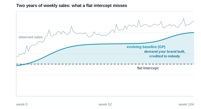
The consequence is a systematic bias, not random noise. Performance channels, whose effects are fast and land inside the model's attribution window, get full credit. Brand channels, whose effects are slow and land in the baseline, get approximately none. Total marketing impact is understated, and the brand-versus-performance split is distorted in a specific, predictable direction. If your budget process treats MMM read-outs as ground truth, this bias compounds year after year: brand looks weak, gets cut, the baseline erodes eighteen months later, and nobody connects the two events.

The baseline is where brand lives

None of this is a new observation. Unobserved Components Models have been used in marketing analytics for well over a decade to let baseline sales evolve, with Cain (2010, 2021) and Thinkbox's Profit Ability study (2018) building long-run marketing measurement on exactly this foundation, and Dekimpe & Hanssens formalising persistence modelling before that. Traditional UCMs describe the base with a local level or local linear trend: flexible, but the parameters governing that flexibility are hard to reason about, and hard to set sensible priors on.

The approach I argued for in 2023, and the one PyMC-Marketing adopted, is to model the baseline with a Gaussian Process instead, using the Hilbert Space GP (HSGP) approximation to keep sampling fast. The practical advantage of a GP is that its two key questions are ones a human can actually answer. How smooth is the baseline, versus how volatile? And over what time scale does it meaningfully change? Those beliefs go directly into the kernel and its length-scale prior. In the original article I suggested constraining the length scale to roughly 4 to 12 weeks: responsive enough to track real shifts in base demand, sluggish enough not to chase weekly noise or steal short-term media effects. That intuition transfers unchanged to the 1.0 workflow.

Stage 1: an MMM with a time-varying intercept

In 2023 this meant writing the GP into a custom PyMC model. In PyMC-Marketing 1.0 it is a constructor argument. You fit an otherwise ordinary MMM on your performance channels, controls, and seasonality, and switch on time_varying_intercept, configuring the HSGP through model_config:

from pymc_extras.prior import Prior
from pymc_marketing.hsgp_kwargs import CovFunc, HSGPKwargs
from pymc_marketing.mmm import MMM, GeometricAdstock, LogisticSaturation

model_config = {
    "intercept_tvp_config": HSGPKwargs(
        m=50, eta_lam=1.0, ls_mu=5.0, ls_sigma=10.0,
        cov_func=CovFunc.Matern52,
    ),
    "intercept": Prior("Normal", mu=4, sigma=1),
    "adstock_alpha": Prior("Beta", alpha=2, beta=3, dims="channel"),
    "saturation_lam": Prior("Gamma", mu=2, sigma=0.5, dims="channel"),
}

mmm = MMM(
    date_column="date",
    target_column="y",
    channel_columns=channels,   # performance channels only
    adstock=GeometricAdstock(l_max=l_max),
    saturation=LogisticSaturation(),
    yearly_seasonality=2,
    time_varying_intercept=True,
    model_config=model_config,
)
mmm.fit(X, y)

Note what is deliberately missing from the channel list: brand spend. Stage 1 is not trying to measure brand. It is trying to do two other jobs well: give performance channels a clean short-term read, and recover the evolving baseline series with full posterior uncertainty. That baseline, extracted from the fitted model, becomes the outcome variable for stage 2. The length-scale prior (ls_mu, ls_sigma) is where the smoothness judgement lives, exactly as with the hand-built GP.

Stage 2: a Bayesian VARX over the funnel

Stage 2 takes the baseline from stage 1 and puts it in a system of equations alongside brand-tracking metrics, typically awareness and consideration from your brand tracker. Each variable is modelled as a function of the previous period's values of every variable in the system, with brand spend entering as an exogenous driver. Conceptually, it is the same system I wrote down in 2023:

Baseline[t]  = a0 + γ1(BrandSpend[t]) + φ11(Baseline[t-1]) + φ12(Awareness[t-1]) + ε1[t]
Awareness[t] = b0 + γ2(BrandSpend[t]) + φ21(Baseline[t-1]) + φ22(Awareness[t-1]) + ε2[t]

The lag structure is the whole trick. Because every variable feeds every other variable with a one-period delay, the system can represent chains like "brand spend lifts awareness now, awareness lifts consideration next month, consideration lifts baseline demand the month after", and crucially, it can represent those effects persisting and compounding rather than decaying on an adstock schedule chosen in advance.

VARs have a well-known problem in marketing: brand metrics arrive monthly at best, so the time series are short and a freely-estimated VAR eats degrees of freedom for breakfast. The answer, then and now, is Bayesian shrinkage. The PyMC-Marketing workflow uses the impulso library with a Minnesota prior, the standard macroeconometric device that shrinks the system toward simple persistence unless the data argue otherwise:

from impulso import VAR, MinnesotaPrior, VARData
from impulso.samplers import NUTSSampler

var_data = VARData.from_df(
    varx_df,
    endog=["awareness", "consideration", "baseline"],
    exog=["brand_spend"],
)

varx = VAR(lags=1, prior=MinnesotaPrior(tightness=0.5, cross_shrinkage=1.0))
fitted = varx.fit(var_data, sampler=NUTSSampler(nuts_sampler="nutpie"))

Two things in the 1.0 workflow are genuine upgrades on what I could offer in 2023. First, diagnostics: the notebook runs Granger-causality checks to validate the assumed funnel ordering rather than taking it on faith. Second, and more important, uncertainty propagation: stage 2 is refit across draws of the stage-1 baseline posterior, so the final long-term ROI carries both the uncertainty about what the baseline was and the uncertainty about how brand moves it. The 2023 version passed a point estimate between stages and quietly understated its error bars. The 2026 version does it properly.

From impulse responses to long-term ROI

With the system estimated, you ask it the question every brand marketer actually cares about: if we spend an extra unit on brand this week, what happens, everywhere, over the next six months? Formally this is an impulse response: shock the exogenous variable once, and trace the ripple through the system week by week as awareness jumps, consideration follows, baseline demand lifts, and the whole thing gradually decays.

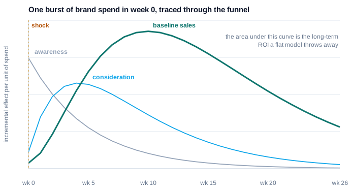
Summing the baseline response over a horizon gives a cumulative dynamic multiplier: total incremental sales per unit of brand spend. In the notebook's simulation, where the ground truth is known because the data are generated, the numbers land like this:

The total value of marketing then decomposes cleanly, as in the original article, into a short-term component read from the MMM and a long-term component read from the impulse responses:

Short-term uplift = Σ media effects from the stage-1 MMM
Long-term uplift  = Σ BrandSpend × IRF(Baseline), summed over the horizon
Total marketing ROI = short-term + long-term

Everything is posterior draws, so each of those lines comes with credible intervals rather than a single number, and the horizon is an explicit choice you can defend (26 weeks in the notebook) instead of an artefact of adstock decay.

What this changes for budget decisions

• The brand-versus-performance split stops being an act of faith. Long-term brand ROI becomes a measured quantity with uncertainty, arguing on the same quantitative footing as performance channel ROIs, instead of a belief defended with case studies.
• Performance plateaus get a diagnosis. When performance marketing efficiency decays over time, the missing variable is often the baseline that brand was quietly feeding. A model that watches the baseline move can see the erosion coming, not just explain it afterwards.
• Scenario questions become answerable. "What happens if we cut brand spend for two quarters?" is exactly an impulse-response question, run in reverse. The system predicts the slow baseline decline that a flat-base MMM is structurally incapable of forecasting.
• Your brand tracker earns its keep. Awareness and consideration stop being a dashboard nobody links to revenue and become load-bearing variables in the measurement system.

Three years from blog post to library feature

In 2023, the honest pitch for this workflow was: the method is sound, the references go back decades, but you will need someone to build it for you. In 2026 the pitch is: pip install pymc-marketing and open the long-term brand effects notebook, which walks the full two-stage workflow on simulated data with known ground truth, so you can verify it recovers the answer before trusting it on your own data. That shift, from bespoke consulting artefact to reproducible open-source workflow, is what open science in marketing measurement is supposed to look like.

The original 2023 article is still up at 1749.io if you want the earlier framing and the full reference list (Cain 2010, 2021; Thinkbox 2018; Dekimpe & Hanssens 2003; Zivot & Wang 2003). For what else landed in the 1.0 release, sampling speedups, multidimensional MMM by default, and three other new workflows, see our PyMC-Marketing 1.0 write-up, and we track the upstream project live on our PyMC-Marketing page.

If your MMM currently tells you brand ROI is zero and your instinct says otherwise, your instinct is probably right and your baseline is probably flat. Book a call and we can look at what a long-term measurement setup would take with your data.