Some MMM convergence problems are obvious. Four chains sit in different places, R-hat is nowhere near one, effective sample size collapses, and divergences arrive by the hundred.
The harder problem is deciding what to change next.
A common workflow is still:
- Guess that a hierarchy is too loose.
- Tighten one prior.
- Run NUTS for hours.
- Discover whether it helped.
- Repeat.
That is a painfully expensive way to tune a complicated hierarchical model.
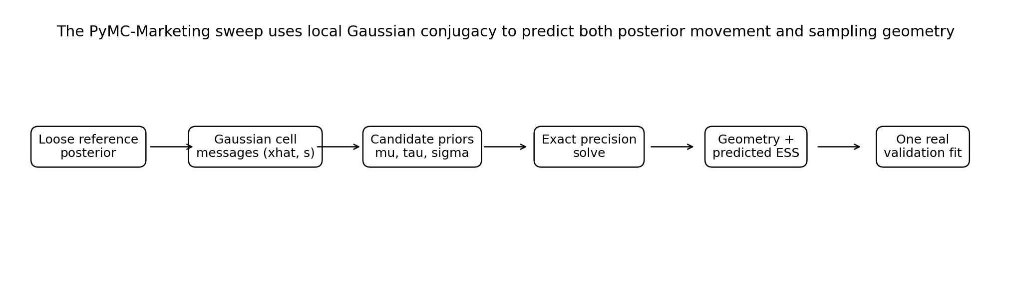
This article shows a different workflow for PyMC-Marketing. We take the analytic prior-sweep machinery from the original refuel approach and generalise it to saved PyMC-Marketing 1.x models. The resulting package predicts two things before the expensive refit:
- how the posterior coefficients should move under a candidate hierarchy
- how the posterior geometry should change, and therefore what NUTS ESS is likely to be, using an empirical calibration from historical sampler runs
The point is not to replace MCMC. The point is to spend MCMC on the candidate that has already earned a validation run.
The case study is deliberately difficult. It contains 60 SKU/customer price coefficients, sparse independent price variation, promotion and price confounding, retailer media that fires with promotional events, a badly shaped centred hierarchy, and a hard upper prior wall on the price hyper-mean. Non-centring helps, but it does not solve the whole problem.
Reproducibility note: the business data are synthetic. The complete case study (14 MB zip) contains a deterministic reference-posterior fixture and deterministic historical ESS anchors so the full article, sweep and figures render without requiring a long MCMC job. The analytic sweep itself is genuinely executed by the bundled package. In a production project, replace the fixtures with a saved PyMC-Marketing reference model and real historical sampler runs.
First, understand the business before blaming NUTS
We are modelling a soft-drinks portfolio across:
- 3 brands: Aster, Brio and Cinder
- 4 variants per brand: Original 330, Zero 330, Original 500 and Zero 500
- 5 customers: NorthMart, ValueHub, CityExpress, FreshBasket and eGrocer
- 156 weeks of weekly data
- 12 SKUs and 60 SKU/customer cells
- 9,360 panel rows
- about 20.0 million synthetic units and 28.2 million synthetic revenue
- TV, paid social, paid search and retailer media
- price, promotion and weighted distribution
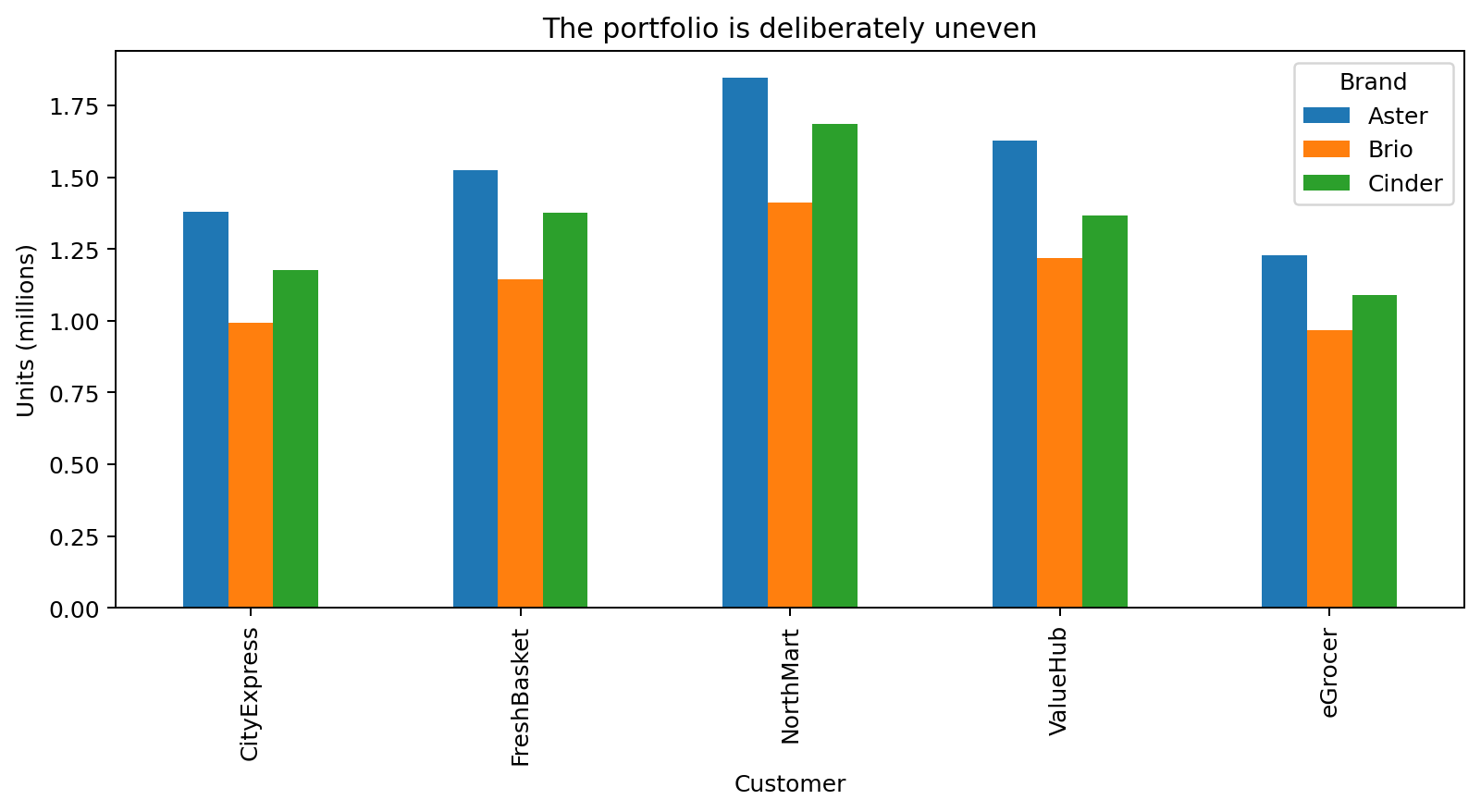
The volume footprint is not balanced. Some customers and brands contribute much more information than others.
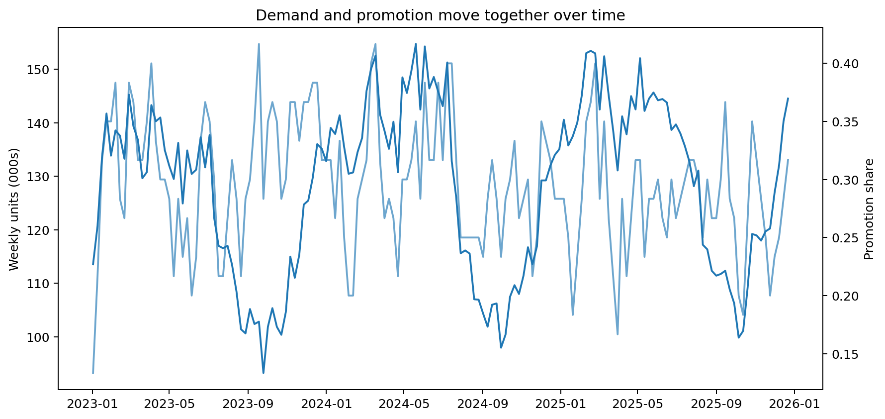
Weekly demand is not stationary either. Promotions arrive in bursts, media pulses through the year, distribution ramps and list price changes gradually.
One difficult cell already contains most of the problem
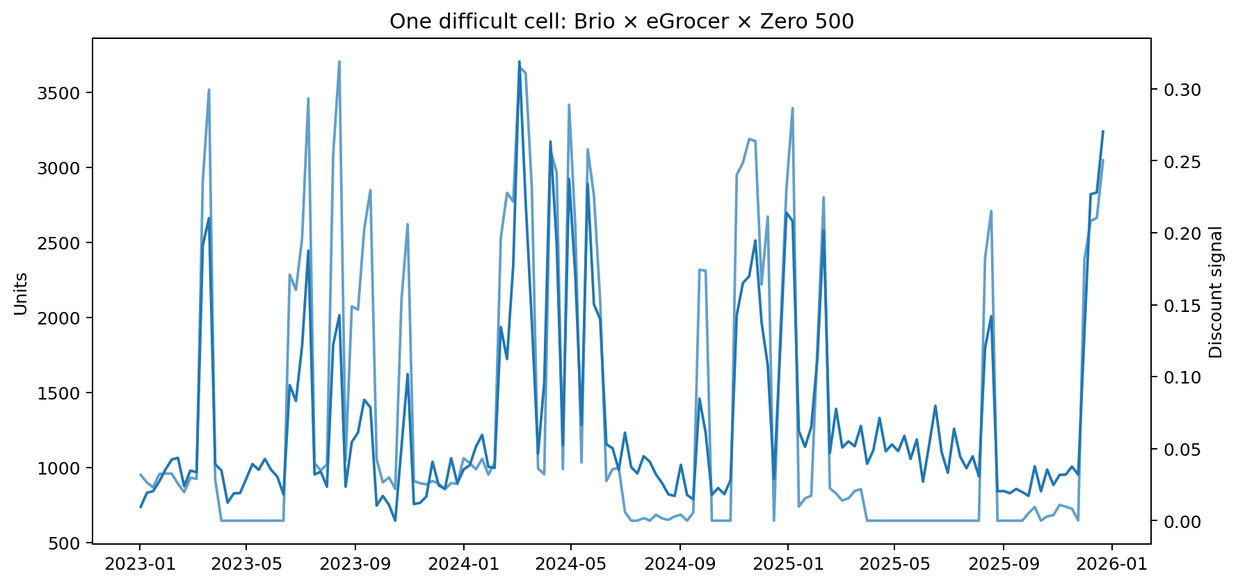
Brio Zero 500 at eGrocer is intentionally awkward. It is price sensitive, online demand is volatile, and most useful price movement happens around a commercial event.
The model uses:
price_discount_signal = -log(actual_price / list_price)A larger value means a deeper effective discount. Because the response is log demand, a positive raw coefficient maps naturally to a negative conventional price elasticity.
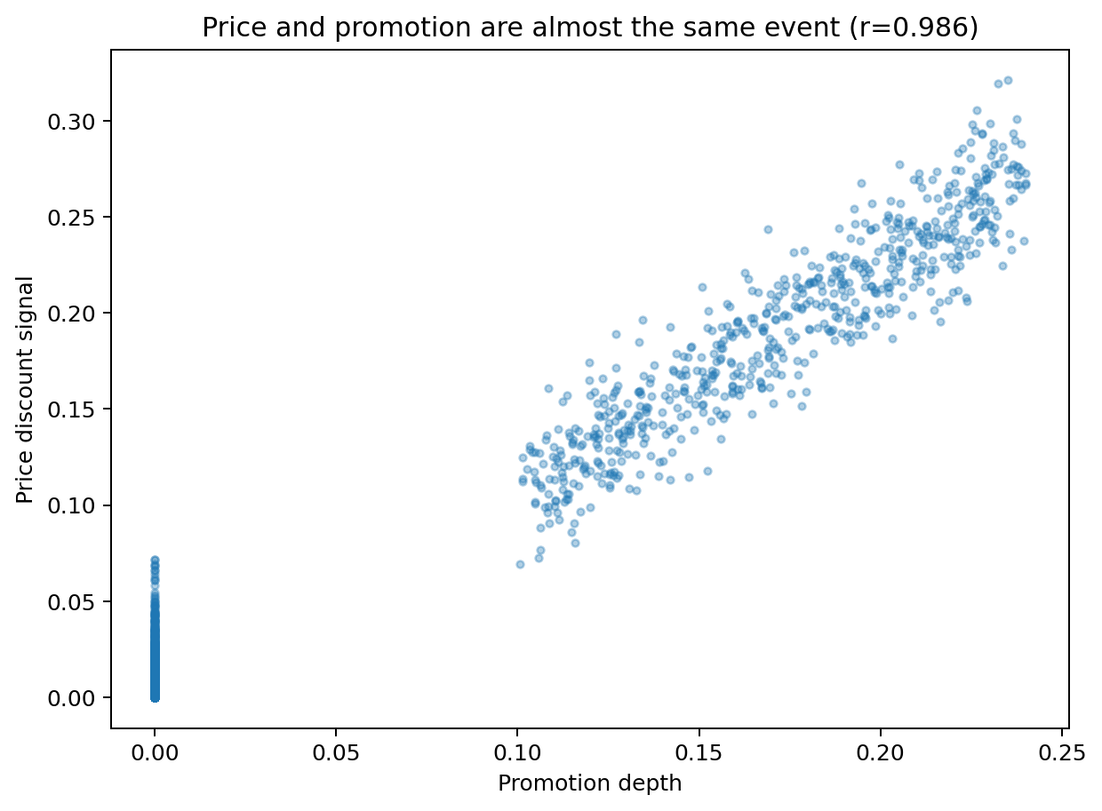
But the price signal is not moving independently. In this synthetic panel, the correlation between promotion depth and the price signal is about 0.986.
Retailer media also fires around those events. The correlation between the price signal and retailer media is about 0.79.
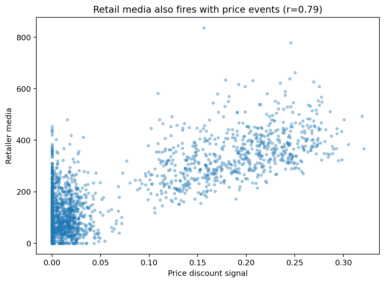
This is why price elasticity is a hard target. The model is not simply learning a clean regression coefficient from independent price experiments.
We still need heterogeneous elasticities
The correct solution is not to collapse the portfolio onto one global price coefficient. The synthetic truth deliberately contains real variation by brand, customer and pack format.
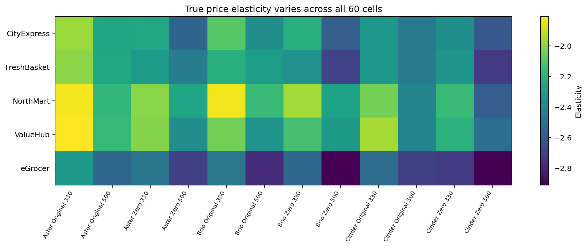
Some cells have almost no independent off-promotion price variation at all.
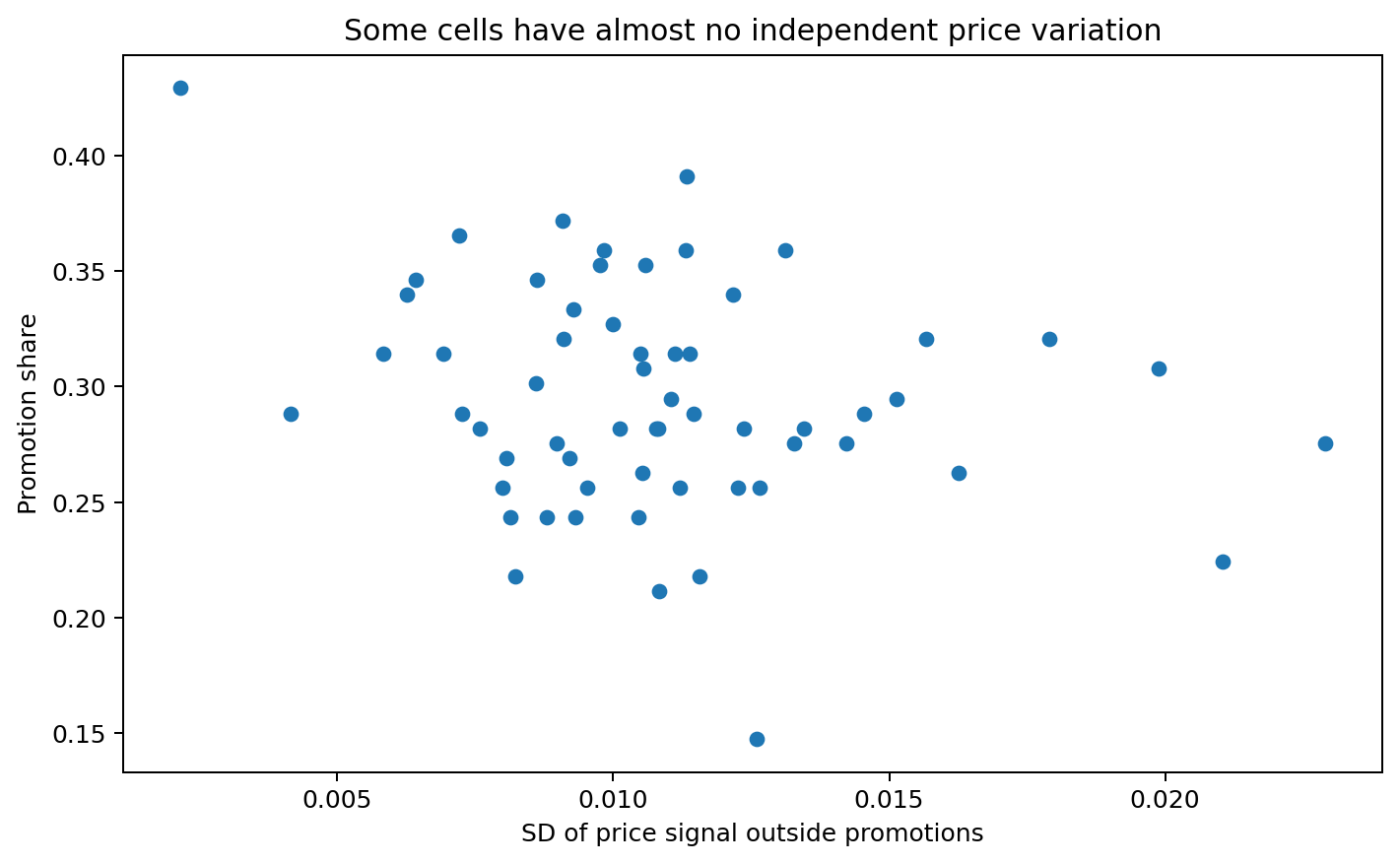
So we want partial pooling. We just do not want a hierarchy whose geometry makes NUTS fail.
The intentionally difficult price hierarchy
The custom PyMC-Marketing model represents the raw price coefficient as an additive non-centred-style block conceptually equivalent to:
price_coef[b, c, v]
    = price_mu
    + sigma_brand   * z_brand[b]
    + sigma_customer* z_customer[c]
    + sigma_variant * z_variant[v]
    + sigma_cell    * z_cell[b, c, v]
with each z having a standard Normal prior.
The initial bad model makes the problem worse in two ways.
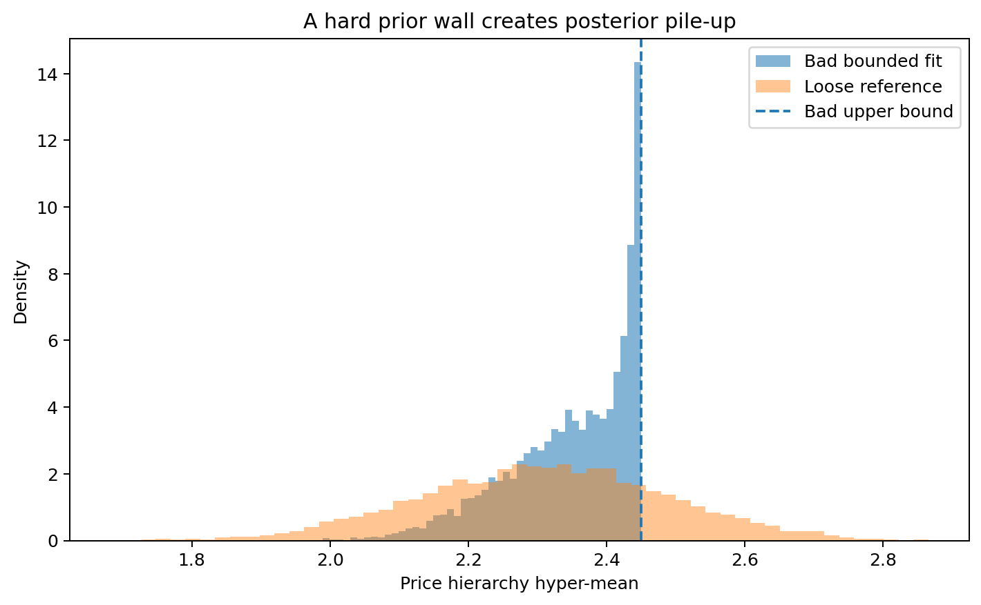
First, the equivalent hierarchy is exposed to the sampler in a centred form. Second, the price hyper-mean is given an upper support wall near an area where the likelihood still wants posterior mass.
That creates a classic interaction between a funnel, a ridge and a boundary.
The model can compensate for a constrained hyper-mean by moving customer effects, variant effects and cell effects. Because price is already confounded with promotion and retailer media, several directions in parameter space can explain almost the same sales pattern.
This is the kind of posterior that looks fine in model code and horrible to Hamiltonian Monte Carlo.
What non-convergence actually means
When four MCMC chains are run, all four are supposed to explore the same posterior distribution. They may begin in different places, but after warm-up they should become exchangeable samples from the same target.
Non-convergence means that has not happened.
The most useful diagnostics tell different parts of the story:
| Diagnostic | What it asks | Failure pattern |
|---|---|---|
| Trace plot | Are chains moving through the same region? | Chains sit at different levels or get stuck |
| R-hat | Is between-chain variation compatible with within-chain variation? | Materially above 1, with roughly 1.01 a common warning line |
| Bulk ESS | How many approximately independent draws do we really have? | Thousands of nominal draws may contain only a handful of useful draws |
| Divergences | Did Hamiltonian trajectories fail in difficult geometry? | Repeated divergences indicate important regions may not be explored correctly |
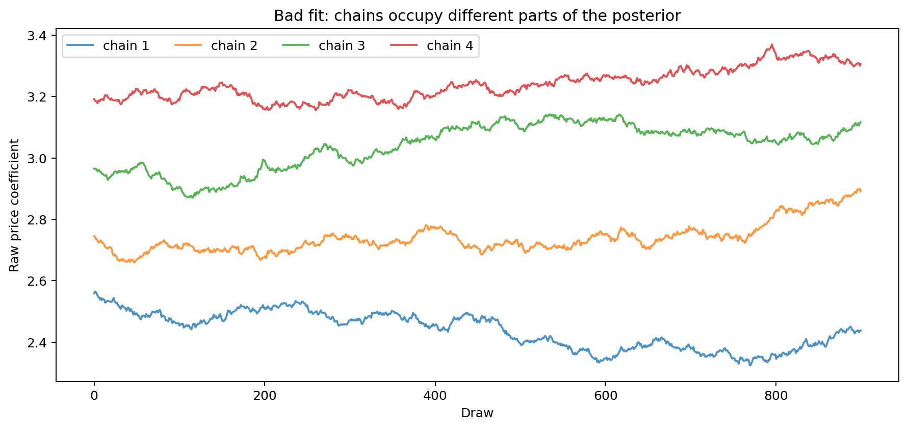
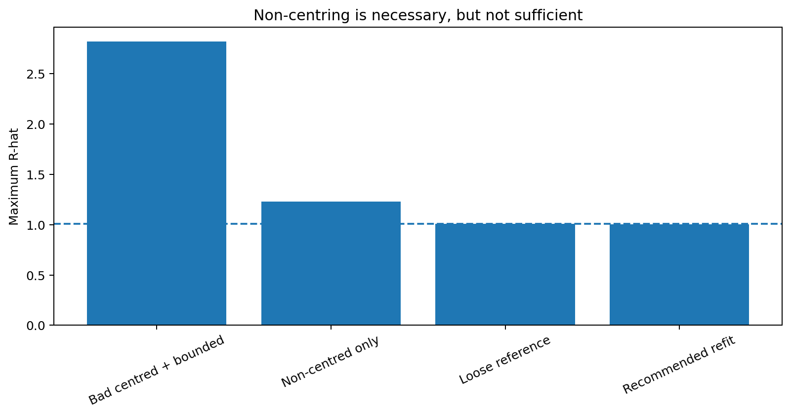
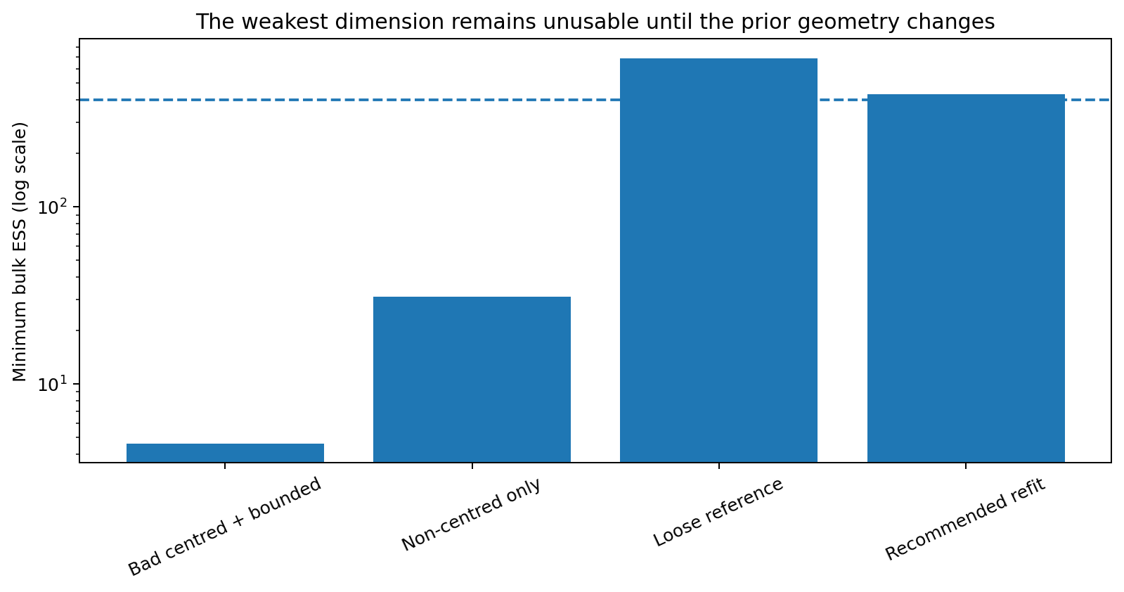
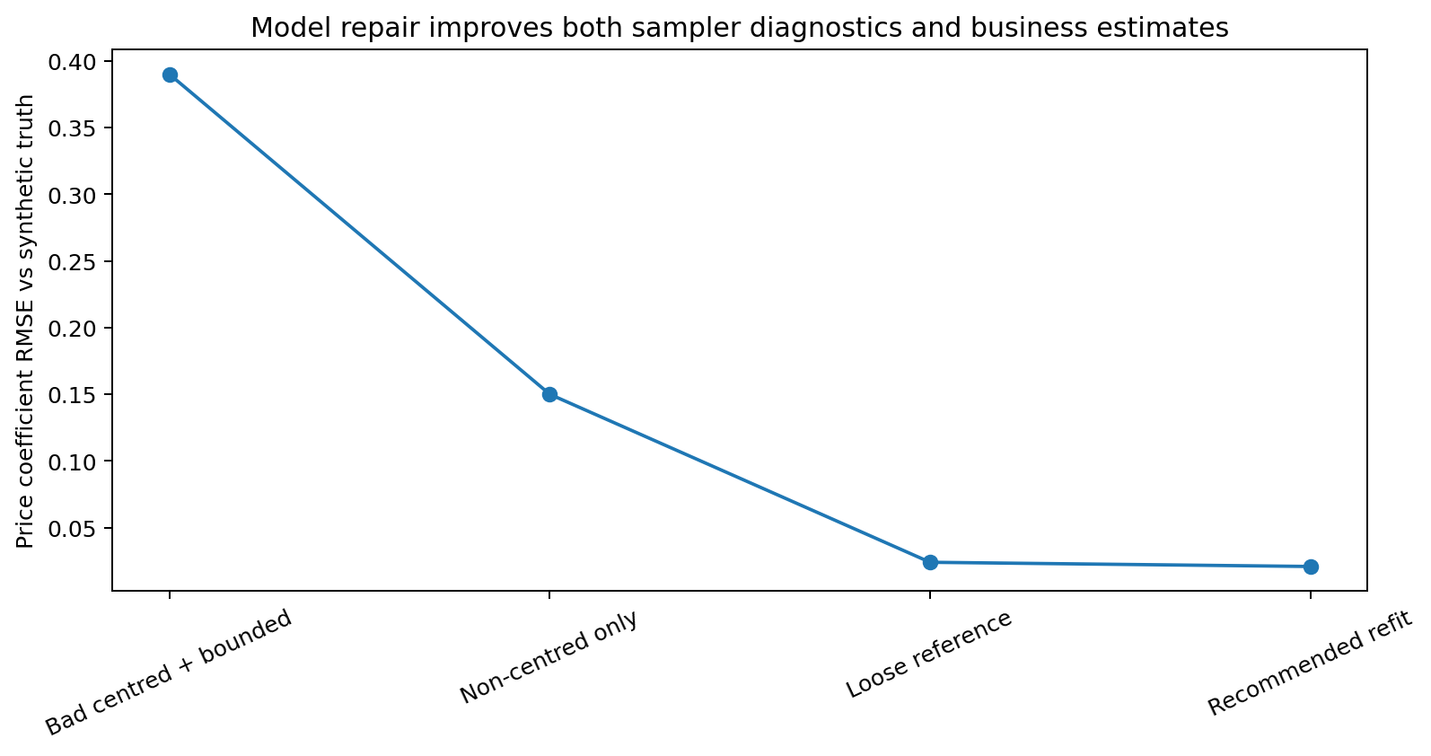
The deliberately bad fixture has 326 divergences, maximum R-hat around 2.82, and minimum bulk ESS around 4.6.
Here is what one price coefficient looks like.
Ignoring draw order and overlaying the chain-specific posterior densities makes the disagreement even clearer.
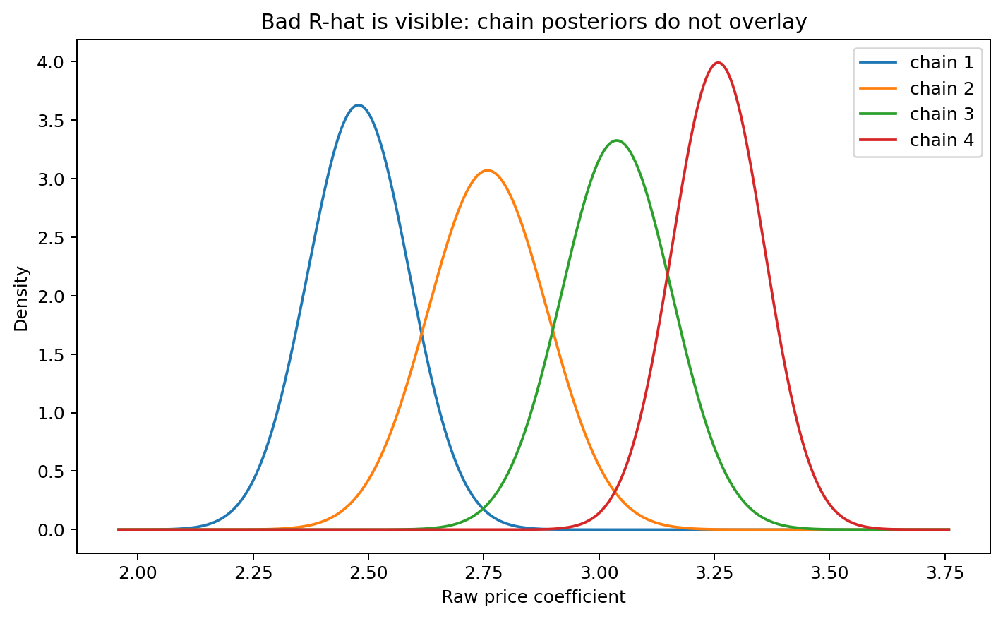
That is what a bad R-hat means in practice. The combined posterior is pretending four incompatible chain-specific answers are one distribution.
Non-centring helps, but it does not fix a bad prior wall
The first repair is still to improve the parameterisation. We switch the hierarchy to a non-centred representation while leaving the commercial likelihood and broad substantive assumptions alone.
That removes much of the funnel geometry.
But it does not solve everything.
The non-centred-only fixture still has:
- 74 divergences
- maximum R-hat around 1.23
- minimum bulk ESS around 31
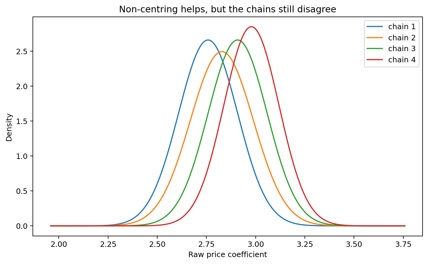
Why? Because a parameterisation change cannot make a bad support restriction disappear.
The price hyper-mean is still pressed against its upper prior wall.
The joint geometry shows the ridge directly.
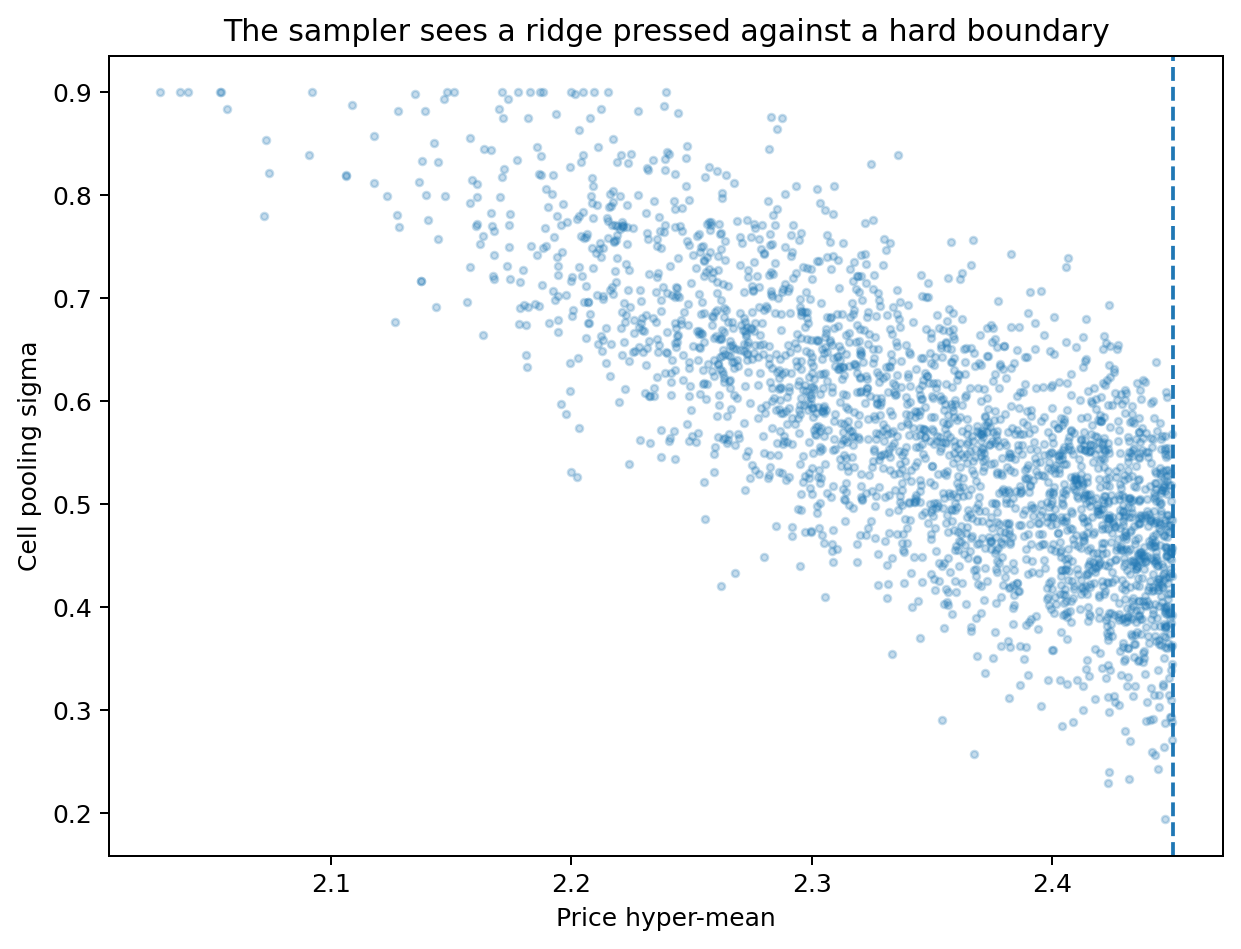
This is the important lesson: non-centring fixes one class of geometry. It does not rescue a prior whose support is fighting the likelihood.
The aggregate diagnostics show the repair stages.
Build one trustworthy loose-prior reference
The analytic sweep needs a trustworthy approximation to the data contribution for each cell.
So we run one diagnostic reference fit with:
- non-centred parameterisation
- a deliberately loose Gaussian hierarchy
- the problematic hard hyper-mean wall relaxed
- a generous sampling budget
- aggressive sampler settings if required
This reference run is allowed to be expensive. It is not the production model we want to deploy. Its job is to learn the local likelihood shape cleanly enough that we can reuse it.
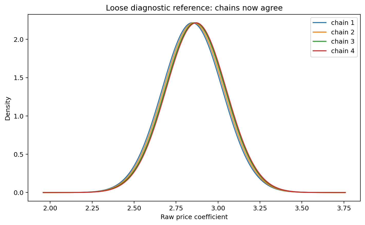
In the fixture, the reference reaches maximum R-hat around 1.006, zero divergences and minimum bulk ESS around 690 despite the deliberately broad design.
The core trick: turn the reference posterior into reusable Gaussian likelihood messages
For each price coefficient cell, the package takes the reference posterior draws and stores only:
xhat = posterior mean
s    = posterior standard deviation
so the data contribution is approximated as:
x_cell | data ≈ Normal(xhat, s)If the reference prior is genuinely loose, this posterior is already close to the likelihood message. The adapter can enforce that assumption with max_prior_information.
If a known scalar Gaussian reference prior is still material, the package can remove it in precision space:
likelihood precision
    = posterior precision - reference-prior precision
This is the point where the original training data disappear from the sweep loop. We have compressed the relevant information into a reusable Gaussian message for each cell.
The PyMC-Marketing adapter does the coordinate work for us. A block configuration declares the real posterior variable and maps PyMC-Marketing dimensions to analytic effects:
block:
  name: price::sku_customer_brand
  posterior_variable: price_coefficient
  cell_dims: [brand, customer, variant]

  intercept:
    name: price_mu
    mu: 2.10
    tau: 0.62

  offsets:
    - name: brand
      source_dims: [brand]
      sigma: 0.34
    - name: customer
      source_dims: [customer]
      sigma: 0.46
    - name: variant
      source_dims: [variant]
      sigma: 0.32
    - name: cell
      source_dims: [brand, customer, variant]
      sigma: 0.30
That same adapter can use geo, DMA, product, customer_segment, or any other dimensions in a custom PyMC-Marketing model.
Solving a candidate prior is just one linear system
Once the likelihood messages exist, the candidate hierarchy is Gaussian.
Write the parameter vector as the intercept plus all standard-Normal raw effects. For every cell, the candidate fixed sigmas appear in the design row r_i.
The posterior precision is:
P = P_prior + Σ_i (1 / s_i²) r_i r_iᵀand the information vector is:
b = b_prior + Σ_i (xhat_i / s_i²) r_iThen:
posterior_mean = solve(P, b)
posterior_cov  = inverse(P)
That is the candidate fit.
There is no NUTS run in the sweep loop.
The scalar price hyper-mean may also have a lower, upper or two-sided bound. Because only one scalar is truncated, the package computes the exact first and second moments of the resulting truncated multivariate Gaussian and reports how close the posterior sits to the boundary.
It deliberately does not pretend arbitrary multivariate hard truncation is conjugate.
How the sweep predicts convergence and ESS
The analytic posterior covariance gives us a correlation matrix. Let its smallest and largest eigenvalues be λ_min and λ_max. The package calculates:
kappa = sqrt(λ_max / λ_min)This is an empirical conditioning metric for the posterior correlation geometry. Higher values mean a more elongated, difficult geometry.
The current production design in this case has kappa ≈ 34.0 with n_free = 72. But kappa alone is not an ESS prediction.
To predict real sampler performance, we use historical PyMC-Marketing runs from the same model family. Each anchor contains the exact prior design, observed bulk ESS and sampling budget. The package reconstructs the analytic geometry for that historical design and fits:
log(ESS / posterior_draws)
    = a + b log(kappa) + c log(n_free + 1)
with Huber robust regression.
Leave-one-run-out residuals provide the prediction interval and a calibration-confidence label.
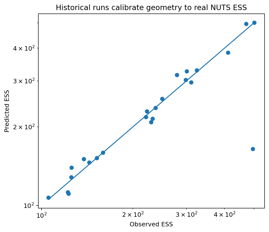
The synthetic story calibration is labelled high confidence. Its leave-one-out log RMSE is about 0.24. One intentionally bad calibration run is downweighted by the robust fit rather than dragging the entire law.
In production, these anchors must be real sampler results. If there are not enough comparable historical runs, the package will not pretend it knows future NUTS ESS.
Now sweep the price hierarchy
The current production design is:
| Prior component | Current value |
|---|---|
| brand scale | 0.34 |
| customer scale | 0.46 |
| variant scale | 0.32 |
| cell scale | 0.30 |
| hyper-mean tau | 0.62 |
| hard upper bound | none in the baseline sweep |
Under the calibrated ESS law, that geometry predicts only about 155 bulk ESS, with an 80% lower bound around 140, at a 6,000-draw posterior budget.
The sweep explores fixed-scale combinations plus several candidate hyper-mean upper bounds. It does not merely maximise ESS. Every candidate must also satisfy coefficient-distortion, prior-data-conflict and boundary guards.
The result is a real trade-off surface.
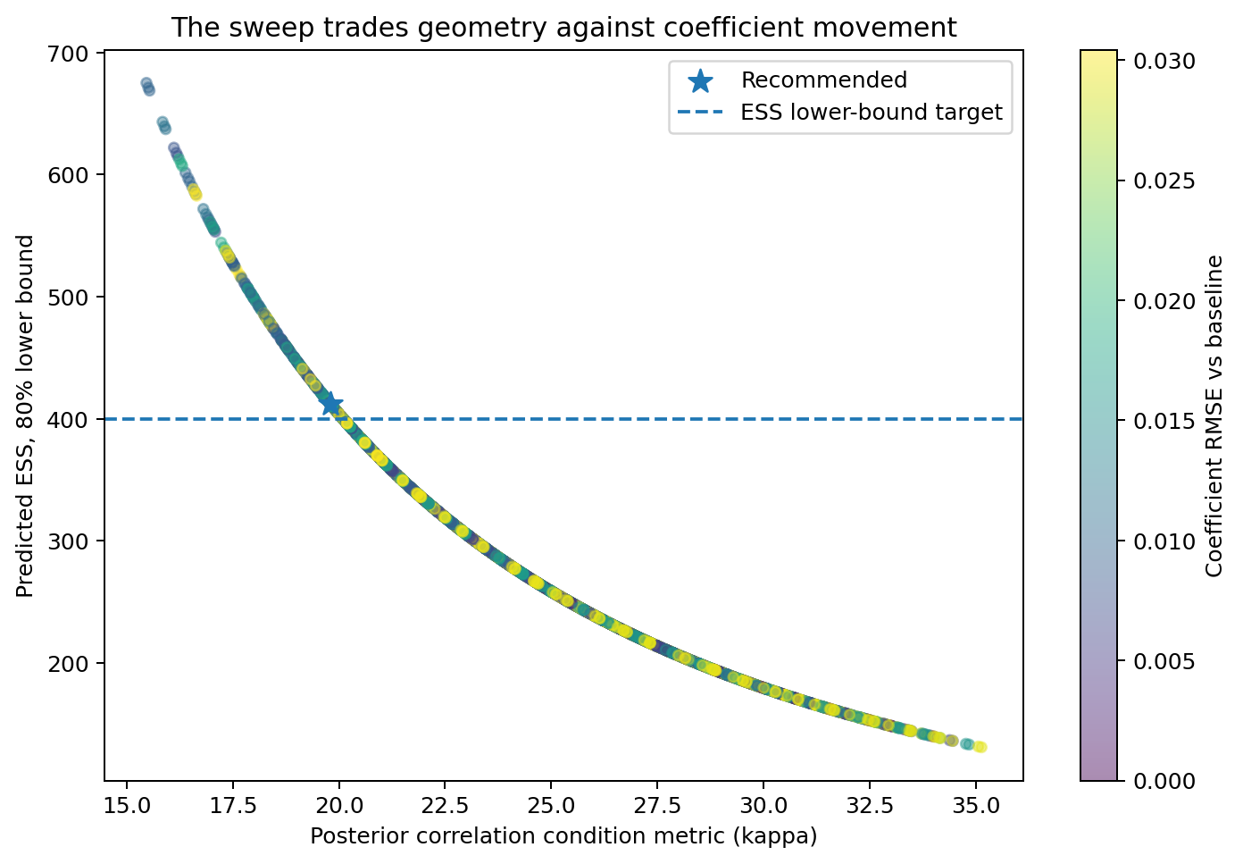
The recommendation
The least-invasive feasible design is:
| Prior component | Current | Recommended |
|---|---|---|
| brand scale | 0.34 | 0.20 |
| customer scale | 0.46 | 0.26 |
| variant scale | 0.32 | 0.18 |
| cell scale | 0.30 | 0.30 |
| hyper-mean tau | 0.62 | 0.62 |
| upper bound | none | none |
Notice what it did not do. It left the cell-level residual scale and hyper-mean tau alone. The sweep found that reducing the higher-level brand/customer/variant flexibility was enough to reshape the posterior without unnecessarily crushing cell-specific variation.
The geometry changes from:
kappa: 34.0 -> 19.8and the calibrated NUTS prediction becomes:
predicted bulk ESS: 458
80% interval:       [412, 508]
The gate uses 412, the lower bound, not the optimistic point estimate.
Coefficient distortion is tiny:
weighted coefficient RMSE vs current design: 0.009
p95 absolute coefficient movement:           0.019
This is exactly what a useful recommendation should look like. Better geometry, a conservative ESS target cleared, and minimal movement in the business quantities.
The coefficient itself changes before we ever refit
This is the part that matters most operationally.
For Brio × eGrocer × Zero 500, the raw price coefficient under the current production design is predicted around 2.859.
Under the recommended hierarchy, the analytic sweep predicts:
raw coefficient: 2.859 -> 2.830
predicted delta:  -0.028
The independent validation-refit fixture lands around 2.871. The synthetic truth is 2.912.
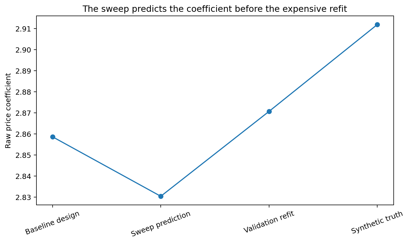
The important result is not that every coefficient moves in the same direction. They should not.
Across all 60 cells, the recommended hierarchy produces a structured pattern of small movements as the higher-level effects pool more strongly.
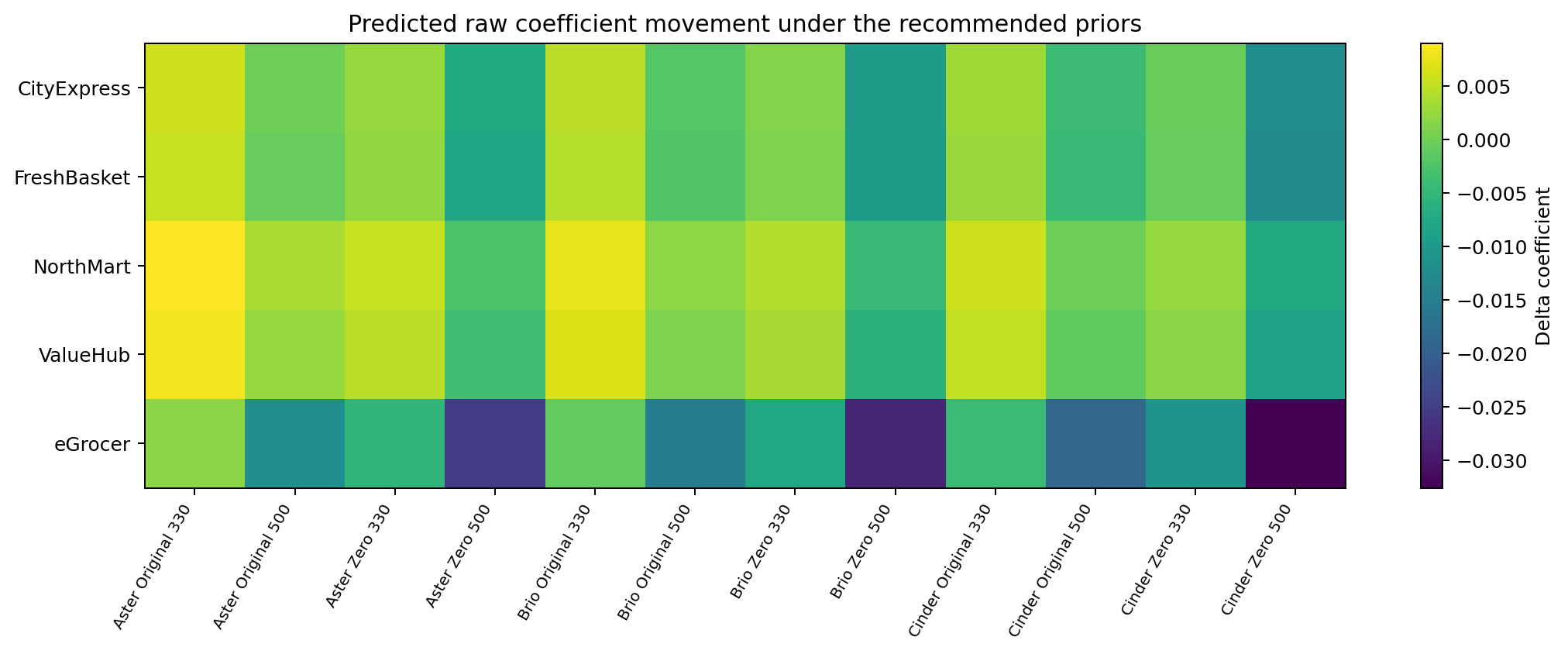
The predicted candidate posterior can be compared directly with the validation refit.
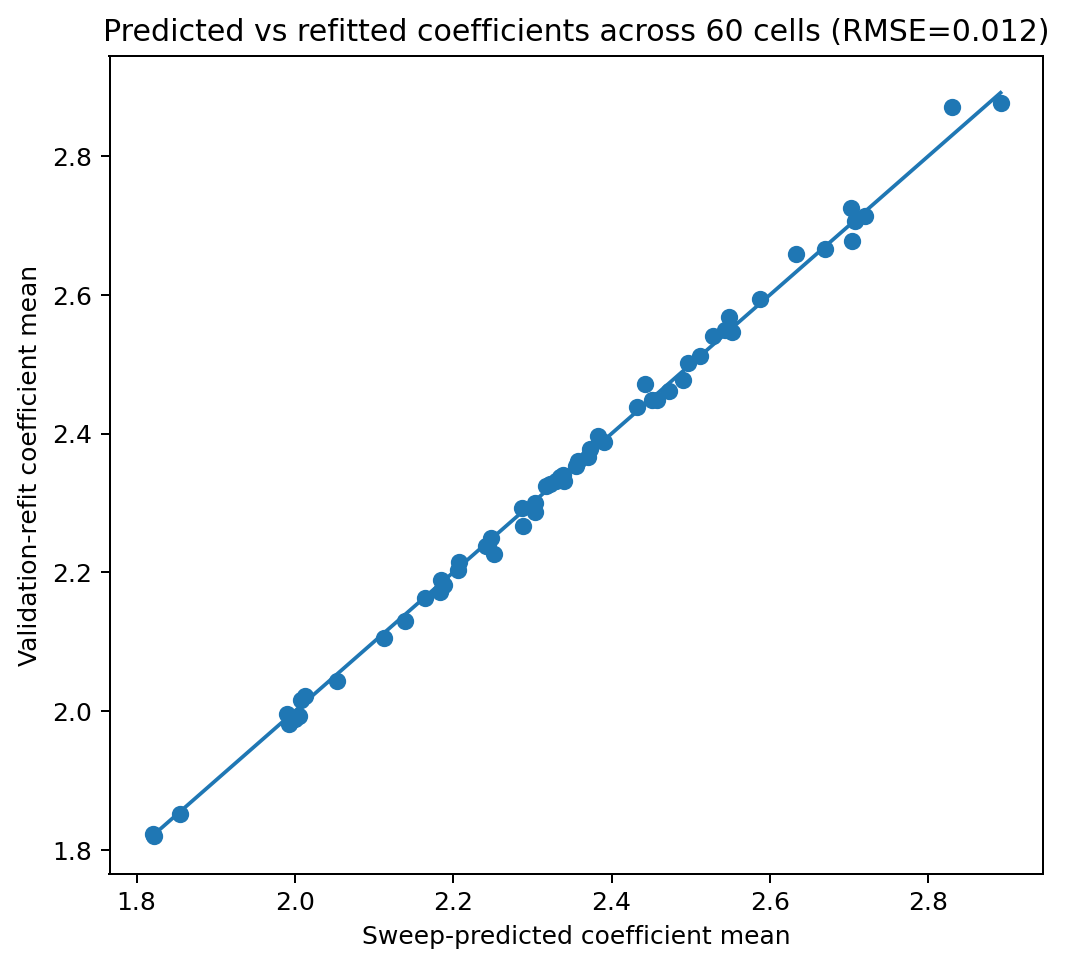
This is the advantage of the conjugate approach over a pure geometry heuristic. We are not only saying “this prior should sample better”. We are predicting the posterior coefficient consequences at the same time.
Bounds are where the story gets interesting
The grid also contains a deliberately aggressive candidate that reintroduces a hard upper bound at 2.45.
The coefficient means hardly move, which might tempt someone to call the candidate safe.
But the geometry tells a different story.
The candidate sits only about 1.47 posterior standard deviations from the upper boundary. Its kappa is about 27.1, and its conservative ESS prediction is only about 220.
It fails both the boundary guard and the ESS target.
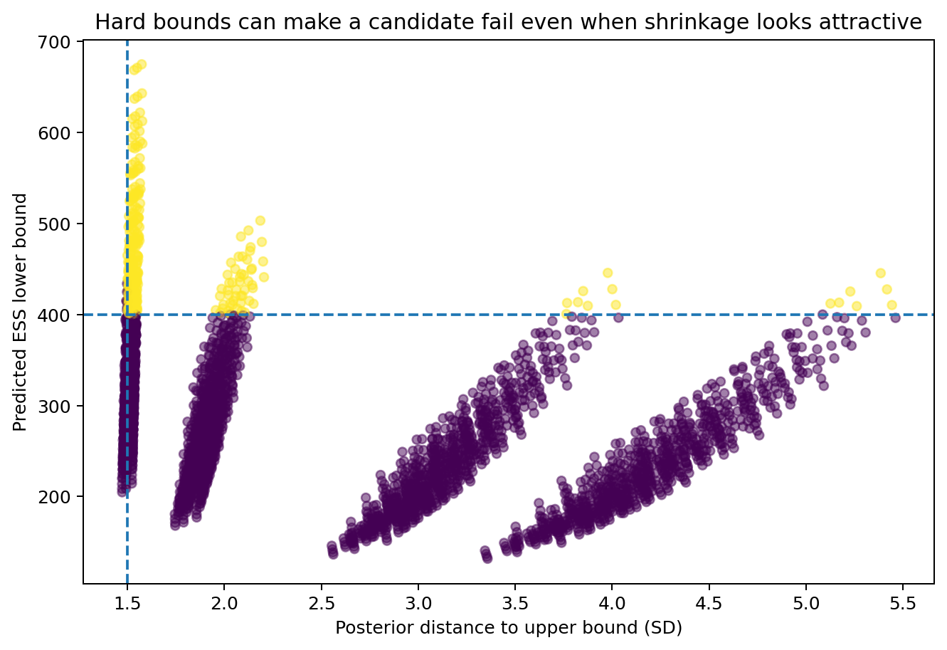
This is exactly the kind of case where “just tighten the prior” is dangerous. A prior can reduce apparent uncertainty while making the Hamiltonian geometry worse.
Does predicted ESS match the actual validation run?
The package should be judged against real sampler behaviour, not only against its own algebra.
The story fixture compares three designs:
| Case | Predicted ESS | 80% lower bound | Observed validation ESS | Kappa | Decision |
|---|---|---|---|---|---|
| Recommended | 458 | 412 | 426 | 19.8 | accept |
| Stronger supported | 495 | 445 | 483 | 19.0 | accept but more invasive |
| Hard-bound candidate | 244 | 220 | 225 | 27.1 | reject |
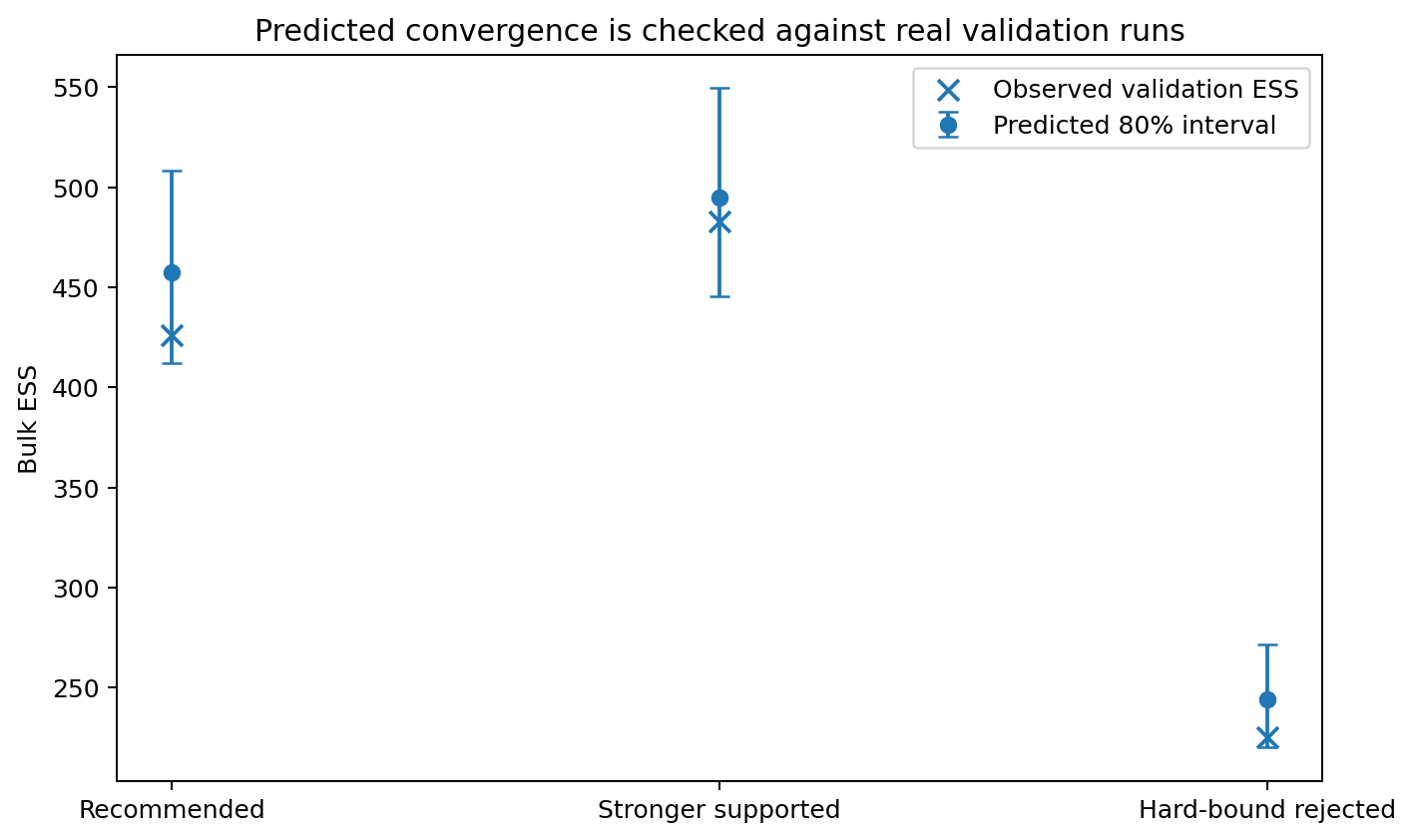
The recommended candidate is not the one with the very highest predicted ESS. It is the one that clears the conservative target with the smallest prior-design change.
That distinction matters. The objective is not “make NUTS as fast as possible”. The objective is “make the smallest defensible model change that produces reliable sampling”.
And what happens to price elasticity?
The raw coefficient is the object the hierarchy directly models. Conventional price elasticity is simply its signed business interpretation in this example.
The validation fit keeps meaningful heterogeneity across customer and SKU while pulling unsupported wandering back towards the hierarchy.
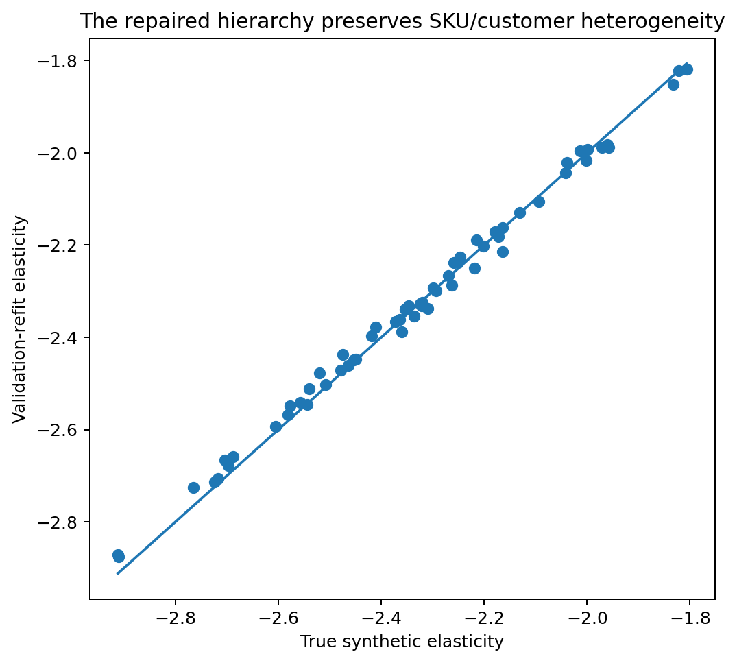
The overall repair path is useful because the sampler diagnostics and business estimates improve together.
Why this is different from a PSIS reweighting sweep
A PSIS prior-reweighting sweep asks whether the existing posterior draws can approximate a new posterior after a prior change.
This package asks a different question.
It first approximates the likelihood contribution of each swept cell as a Gaussian message. Candidate priors are then solved analytically from that prior-independent information.
That has an important consequence: the package can calculate a new candidate covariance matrix and use its geometry to predict NUTS ESS through historical calibration.
In short:
| PSIS reweighting | Analytic Gaussian-message sweep | |
|---|---|---|
| Keeps full reference draws | yes | no, compresses each swept cell to mean + SD |
| Requires conjugate/local Gaussian structure | no | yes |
| Predicts candidate coefficient posterior | yes | yes |
| Explicit candidate covariance/geometry | indirect | yes |
| Predicts calibrated future NUTS ESS | not by itself | yes, with historical anchors |
| Needs historical ESS calibration | no | yes |
| Handles arbitrary prior families | broader | narrower |
| Very fast candidate loop | yes | extremely fast |
For this use case, predicting convergence is the reason to choose the analytic approach.
The package is generalised for custom PyMC-Marketing models
The bundled repository contains a vendor-neutral skill:
pymc-marketing-sweep/
├── AGENTS.md
├── CLAUDE.md
└── .agents/
    └── skills/
        └── pymc-marketing-sweep/
            └── SKILL.md
The skill tells Codex, Claude or Cursor to inspect the custom model before writing a sweep. The agent should discover:
- the saved posterior variable that represents the problematic coefficient
- its actual dimensions and coordinate labels
- the additive Gaussian hierarchy used by the production model
- the fixed sigma values that correspond to each raw effect
- the reference prior looseness
- the historical runs that can be used as ESS anchors
- the model-specific code that turns a recommended generic design back into native PyMC-Marketing configuration
So the dimensions do not have to be brand × customer × variant. They could be country × channel, DMA × product × retailer, or market × brand × pack × customer_segment. The analytic engine does not care about the business names. It cares about the latent Gaussian structure.
A useful agent prompt is:
Read AGENTS.md and the pymc-marketing-sweep skill first.

Inspect my saved PyMC-Marketing 1.x reference model.
Find the latent block that controls the unstable price coefficients.
Do not guess variable names or dimensions.

Map the coefficient posterior into Gaussian cell messages and reconstruct the
current additive non-centred hierarchy as intercept + fixed-scale raw effects.

Use my historical sampler runs to fit the robust ESS law. Reject automatic
recommendations if the calibration is low confidence.

Sweep conservative alternatives around the current mu, tau and fixed sigmas.
Require the 80% lower ESS prediction bound to exceed 400.
Protect price coefficients from excessive movement and reject candidates close
to an active scalar prior boundary.

Return the least-invasive feasible design, the predicted coefficient changes,
the predicted ESS interval, and the exact production-model settings I should
validate with one real NUTS run.
That is a much safer coding-agent task than “change priors until R-hat looks better”.
Running the repository
The repo targets PyMC-Marketing 1.x and Python 3.12+, and everything in this article ships in the case study zip: the data generator, the deterministic fixtures, the figures and the complete pymc-marketing-sweep analytic engine. Create an environment:
python -m venv .venv
source .venv/bin/activate
pip install -e "./pymc-marketing-sweep[dev]"
Fast, fully reproducible article path
The included synthetic fixture can be rebuilt without fitting a full MMM:
python scripts/generate_data.py
PYTHONPATH=pymc-marketing-sweep/src python scripts/generate_story_artifacts.py
python scripts/make_figures.py
python scripts/render_html.py
Or run the complete sequence with ./run_demo.sh.
Real PyMC-Marketing workflow
With a real saved reference model:
pmm-sweep inspect outputs/runtime/reference_model.nc
pmm-sweep run configs/price_sweep.yaml
The run writes:
outputs/runtime/sweep/
├── sweep_predictions.csv
├── recommended_scenario.yaml
├── recommended_model_config.py
├── block_metadata.json
├── ess_calibration.json
└── ess_diagnostics/
The final step is still a real validation fit. Compare:
- observed bulk ESS with
pred_ess,pred_ess_lowerandpred_ess_upper - actual coefficient means and intervals with the analytic prediction
- divergences and R-hat with the expected improvement
- important business outputs with the baseline model
Then add that real validation run as another ESS anchor. The calibration improves as the workflow is used.
What this method can and cannot do
It is powerful because it is narrow.
It works best for swept latent blocks that are locally close to Gaussian and can be represented as fixed-scale Gaussian raw effects plus an intercept/hyper-mean.
It should not be forced onto:
- strongly multimodal latent blocks
- arbitrary multivariate hard truncation
- highly non-Gaussian priors that cannot be represented on the latent Gaussian scale
- models where the ignored cross-block dependence is the main source of geometry
- a reference fit whose posterior was never sampled reliably
- ESS calibrations with too few or incomparable historical runs
When those assumptions fail, the correct answer is not a more confident sweep. It is a real model redesign or refit.
The practical takeaway
A difficult hierarchical MMM often needs two kinds of reasoning at once.
You need to know what the prior change will do to the business coefficients, and you need to know whether it is likely to make the sampler behave better.
The generalised PyMC-Marketing sweep is useful because it puts those two questions in the same table.
For this case:
current kappa:                 34.0
recommended kappa:             19.8
current predicted bulk ESS:    155
recommended predicted ESS:     458
recommended 80% lower bound:   412
coefficient RMSE vs baseline:  0.009
validation observed ESS:       426
The final recommendation is deliberately not dramatic. It tightens the parts of the hierarchy that are creating weak geometry, leaves the cell scale alone, avoids the hard prior wall, and predicts only small coefficient changes.
That is the outcome we want.
Do not ask NUTS to brute-force a badly shaped posterior if you can cheaply predict a better-shaped one first.
SIMBA builds on PyMC-Marketing for transparent Bayesian MMM, including the convergence and diagnostics workflow described here. If your hierarchical MMM will not mix and you want a second pair of eyes, book a call.