Run a decent burst of TV this week and the sales don't all arrive this week. Someone sees the ad on Tuesday, thinks about it, mentions it to a friend at the weekend, and buys three weeks later. Advertising has a memory. Any marketing mix model that ignores that will quietly hand your TV budget's credit to whatever channel happened to be running when the sale finally landed.
MMMs deal with this using something called adstock, old ad-industry jargon for the “stock” of advertising effect you've built up over time. Instead of relating this week's sales to this week's spend, the model relates them to this week's spend plus a fading echo of every previous week. The most popular version, geometric adstock, makes one simple assumption: each week, the echo fades by a fixed proportion. That proportion is the retention rate, α.
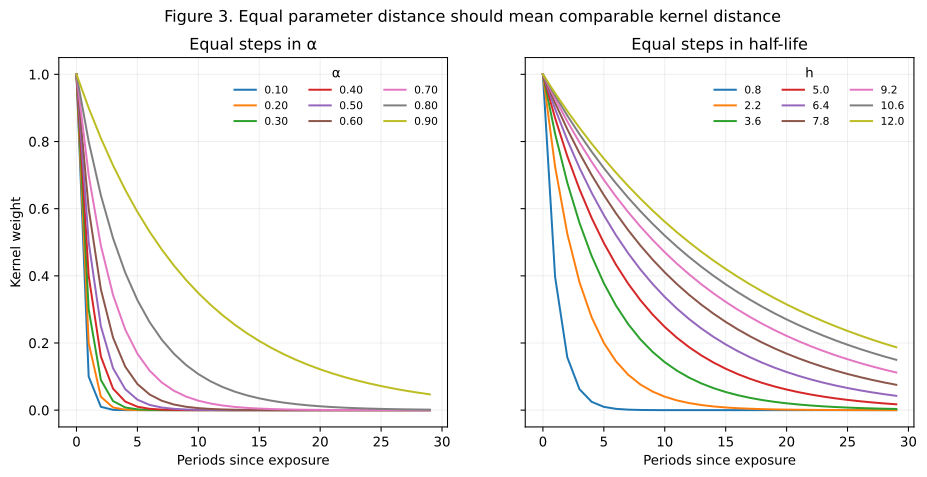
So α = 0.5 means half the effect survives into next week. α = 0.9 means ninety percent survives. Fit the model, read off α, job done. Except that in practice, α is where MMM conversations go to die. I've watched a room of smart marketers nod politely at “TV's alpha came out at 0.93” with nobody, sometimes including the modellers, having any real feel for whether that's plausible. And the confusion isn't the room's fault. The scale itself is broken. Watch what happens when we take two identical-sized steps on it:
The first step is a rounding error. The second quietly adds two months of advertising memory. Same-sized move, 133 times the consequence. The reason: the thing α actually controls, the number of weeks an effect hangs around, is squashed into the very top of the scale. Every long-memory channel you care about (TV, video, anything brand-building) lives crammed up against α = 1, where the third decimal place suddenly matters.
Try it yourself
Honestly, the quickest way to get this is to play with it for ten seconds. Both sliders below control the same decay curve: the top one walks through α at a steady pace, the bottom one walks through the memory itself.
Notice the top slider barely changes the curve for most of its travel, then suddenly changes everything. The bottom slider feels even the whole way; that is the coordinate your intuition lives in.
That “flat, flat, flat, cliff” feeling in the top slider is the whole problem in miniature. It's also why a tidy-looking model result such as α = 0.96 ± 0.01 can hide enormous uncertainty about the thing you actually wanted to know. The same ± 0.01 around α = 0.30 means basically nothing.
There's a better word for this, and physics got there first
The friendly way to describe something that fades by a constant proportion is its half-life: how long until it drops to half strength. Same maths as radioactive decay. “TV's effect halves in about ten weeks” is a sentence a brand manager, a finance director and a statistician can all argue about over one coffee. “TV's α is 0.93” is not, even though it's the same claim.
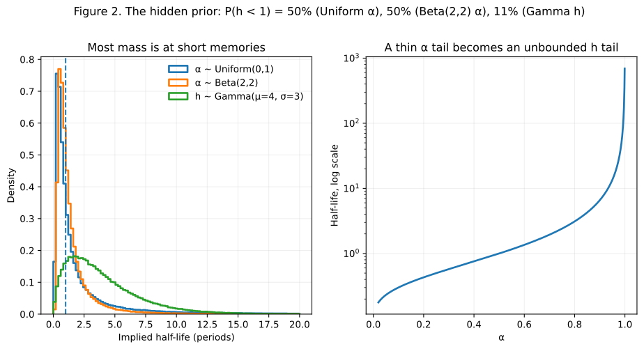
This matters more than it sounds, because a Bayesian MMM runs on prior knowledge, and the knowledge genuinely exists. Your media team roughly knows how their channels decay: search burns out in days, TV lingers for months. But that knowledge lives in weeks. If the model demands it as a distribution over α, you're forcing a translation through the hockey stick, and the hockey stick mangles it. The classic “play it safe” choice (a flat prior over α, every value equally likely, surely harmless) is the best example. Translate it back into memory units and look at what it actually claims:
Half of that “neutral” prior's belief is that advertising is forgotten inside a single week. Nobody at your company believes that. Nobody chose it, either; it just fell out of a coordinate change no one looked at. (And the Beta(2,2) prior some tools default to isn't much better: its median implied half-life is still one week.) Compare that with simply saying what you mean in time units: “probably around a month, give or take a few weeks”, which is a perfectly ordinary Gamma prior on the half-life itself.
The fix is two lines of code
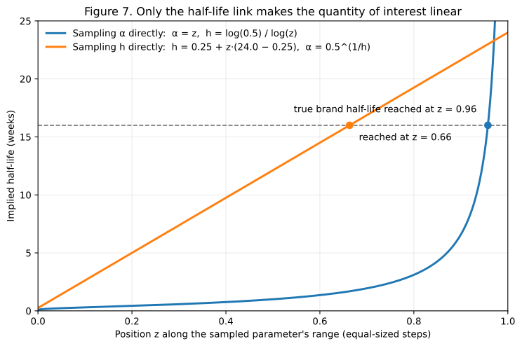
Put the prior on the half-life directly, in weeks, and compute α from it. If h is the half-life, then α = 0.51/h, which is just the definition of a half-life turned inside out. In PyMC:
half_life = pm.Gamma("half_life", mu=4.0, sigma=3.0)  # in weeks
alpha = pm.Deterministic(
    "alpha",
    pt.exp(pt.log(0.5) / half_life),
)
# Feed alpha into your existing geometric adstock, unchanged.
The adstock calculation itself doesn't change at all; α still gets fed into the same formula it always did. What changes is who can join the conversation. “Ten weeks feels too long for this campaign” is an objection a brand manager can raise in a meeting and a modeller can act on the same afternoon. “Beta(1,3) feels too strong on α” is a conversation that has never happened in the history of marketing.
Numbers your team can argue with
For weekly data, here's the kind of opening bid we'd put on the table: not defaults to obey, just numbers for your team to disagree with. That disagreement is the point: it's how the knowledge in people's heads gets into the model.
| Channel class | Plausible half-life | Example prior |
|---|---|---|
| Search or performance | 0.5 to 3 weeks | Gamma(μ=1.5, σ=1) |
| Social or display | 1 to 6 weeks | Gamma(μ=3, σ=2) |
| TV, video or brand | 4 to 26 weeks | Gamma(μ=10, σ=6) |
| Trade or promotion | 0.5 to 2 weeks | Gamma(μ=1, σ=0.5) |
Checking what a prior like this implies takes a few lines:
rng = np.random.default_rng(42)

shape = (4.0 / 3.0) ** 2
scale = 3.0**2 / 4.0
half_life_draws = rng.gamma(shape=shape, scale=scale, size=20_000)
alpha_draws = 0.5 ** (1.0 / half_life_draws)

lags = np.arange(52)
kernels = alpha_draws[:, None] ** lags[None, :]
Working in time units keeps paying off as the model grows, too. Want to share information between similar channels, or encode a belief like “brand memory outlasts performance memory”? In half-life space those are ordinary, checkable statements about weeks. In α space their practical meaning warps depending on where you are on the scale.
It makes the sampler's job easier too
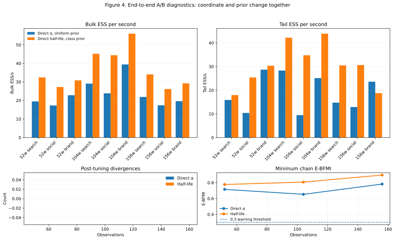
There's a computational side to this as well, and it bit us in our own benchmark. The sampler behind PyMC explores the space of plausible parameter values by taking steps, and it works best when a step of a given size means roughly the same thing everywhere. You can guess the problem: with a flat prior on α, every long-memory model is crammed into that razor-thin sliver below α = 1. The sampler needs microscopic steps there and big ones everywhere else, can't do both, and starts throwing warnings (the dreaded divergences) while producing fewer usable samples.
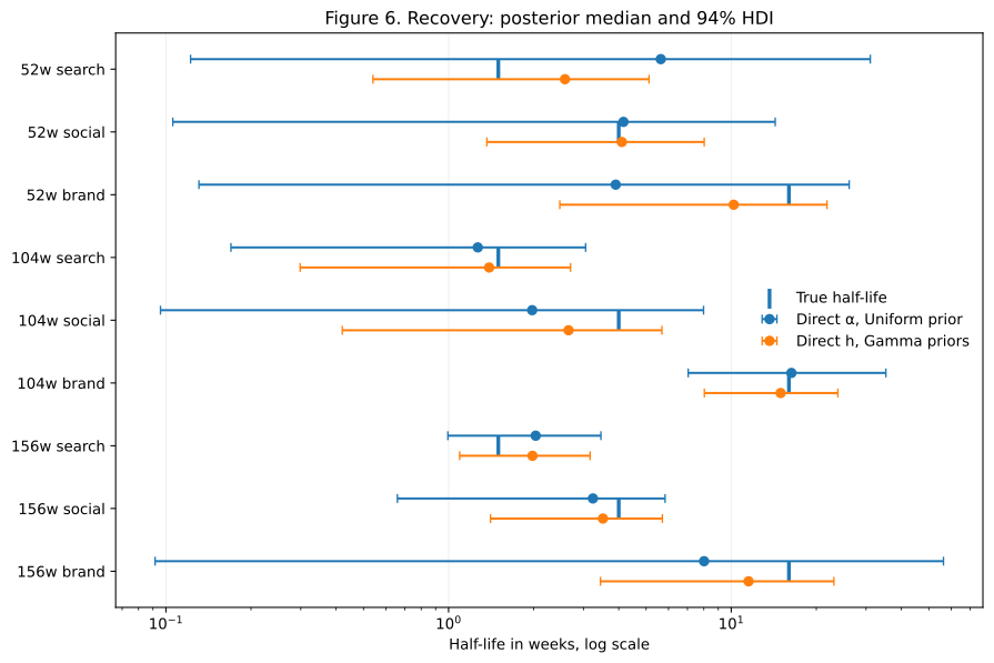
We tested this properly on simulated weekly data: three channels with known true half-lives of 1.5, 4 and 16 weeks, at one, two and three years of history, everything identical between the two versions except the adstock prior. Our first pass, at PyMC's usual settings, made the point loudly: the flat-α model sprayed 107 divergence warnings on the three-year run (and the half-life model wasn't spotless either, with ten). Divergences are curable if you're willing to pay for them, so for the results below we turned the sampler's caution up (target_accept=0.97, slower and more careful stepping) until everything ran clean. At those settings the half-life model recorded zero divergences at every dataset size. But careful stepping costs time, and it can't fix what a prior believes. Here's the three-year run:
And the flat-α model's actual answers were as shaky as its warnings suggested. For the brand channel, where we know the true half-life is 16 weeks because we simulated the data, it technically “covered the truth,” but only by being uselessly vague:
“Somewhere between no memory and a year” is not an answer you can plan a media budget around. And when a model's median and mean are telling you stories that different, neither one deserves your trust. Meanwhile the half-life version, on exactly the same data, pinned all three channels down with intervals you could actually use:
Being honest about why it works
We wanted to know whether the magic was in the half-life coordinate itself or just in having a sensible prior at last. So we ran a control: same three years of data, sampling α directly again, but this time carrying the half-life prior across to the α scale exactly (for the technically minded: including the Jacobian). Result: close. The good prior did most of the work regardless of which coordinate carried it, though sampling half-life directly did keep a modest edge, running clean where the control still produced a few divergences, and getting noticeably more effective samples per second.
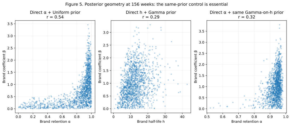
So the honest conclusion is: the big win came from replacing an accidental prior with a deliberate one. Half-life isn't computational magic; it's the coordinate that makes deliberate priors easy to state, easy to defend, and easy to reuse. Which, given how the accidental prior got there in the first place, is exactly the fix that was needed.
The fine print
- Reparameterisation can't create information. If the data can't tell an 8-week memory from a 16-week one, the posterior should stay wide; half-life just makes that honesty visible in useful units.
- Respect the truncation window. A half-life near or beyond
l_maxcan't be expressed by the implemented kernel. Extendl_max, bound the prior, or both. Don't put prior mass where the kernel can't follow. - Check conventions. We treat α as retention (higher = slower decay); some APIs use a decay rate running the other way. And daily vs weekly data changes the numbers, not the argument.
One more practical note: as of August 2026, the big MMM tools all still hand you the raw coordinate. PyMC-Marketing's geometric adstock takes a direct α with a Beta(1,3) default, Robyn optimises a direct θ, and Meridian samples a direct α with a Uniform(0,1) default. None of them is wrong to do so, but it does mean the translation job lands on you. Before trusting any α prior, including a default, check what it secretly says about memory.
Make half-life the parameter
So: talk about adstock in half-lives. Set your priors in half-lives. Report your results in half-lives. Let α become a two-line implementation detail that feeds the same formula it always did. It costs almost nothing, and it turns “α is 0.94” into “the effect halves every eleven weeks”, a sentence everyone in the room can understand, challenge, and improve. That last part is where better models actually come from.
And if geometric adstock is not the shape you want? The argument survives the change of curve. We work through the delayed case, where the same trick buys you a peak time as well as a width, in the follow-up: Half-Life Is Still the Parameter.
SIMBA builds on PyMC-Marketing for transparent Bayesian MMM. If you want to talk through adstock priors for your own channels, book a call.