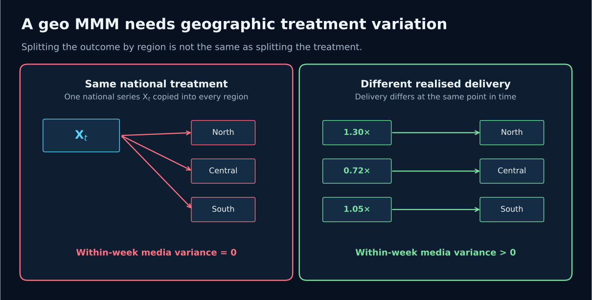
The fast answer: a geo MMM is a causal upgrade only when realised media exposure differs across regions at the same point in time. Splitting the outcome by region does not split the treatment, and allocating national spend by population share invents variation that vanishes the moment you put spend on a per-person scale. Before building the hierarchy, measure how much channel variance survives after removing region means and week means. If the answer is none, keep national channels national and use a hybrid structure.
A regional MMM sounds like an obvious upgrade. More rows. More granular sales. More local controls. A hierarchy that can partially pool information across regions. What is not to like?
One thing matters before all of that: did the treatment actually vary by region?
If a TV campaign, sponsorship or other national buy gives every region the same media time series, then geography has not created a new media comparison. You may have better information about regional baseline demand, but the media effect is still being identified from national time variation.
That distinction is easy to miss because a panel dataset looks richer than a national time series. It has thousands of rows instead of hundreds. But causal information is not measured in row count. It comes from useful variation in treatment.
Google’s 2017 paper on geo-level Bayesian hierarchical MMM makes almost exactly this point. The authors attribute the gain from geo models to more observations and useful variability in media spend, and report that estimates generally deteriorate as more geo media variables are imputed from national-level data. Sun et al., 2017, Google Research
The fast answer, case by case
| Situation | Is a geo MMM causally useful? | Why |
|---|---|---|
| Spend or realised exposure genuinely differs by region at the same time | Yes, potentially | The model gets a cross-sectional treatment contrast in addition to time variation. |
| Sales are regional, but each region receives the same national media series | Not as a media identification upgrade | Geography can model baseline differences, but it adds no new cross-sectional media contrast. |
| National spend is split to regions using population shares | No | The split is invented. It changes accounting labels, not treatment. |
| Media is bought nationally but impressions, reach or delivery vary by region | Possibly | Use the observed regional delivery. The buy may be national while the realised treatment is not. |
| Some channels are national and others are local | Use a hybrid | Keep national treatments national and use geo structure where exposure genuinely varies. |
The strongest version of the rule is not “never build a geo model for national buying”. It is: do not treat geographic outcome granularity as geographic treatment variation.
What a geo MMM is actually buying you
Start with a deliberately simple panel model:
gindexes regions andtindexes time,αgcaptures persistent regional differences,λtcaptures shocks common to all regions at a point in time,xg,tis regional media exposure, andf(·)can include adstock and saturation,zg,tcontains regional controls such as price, distribution or weather.
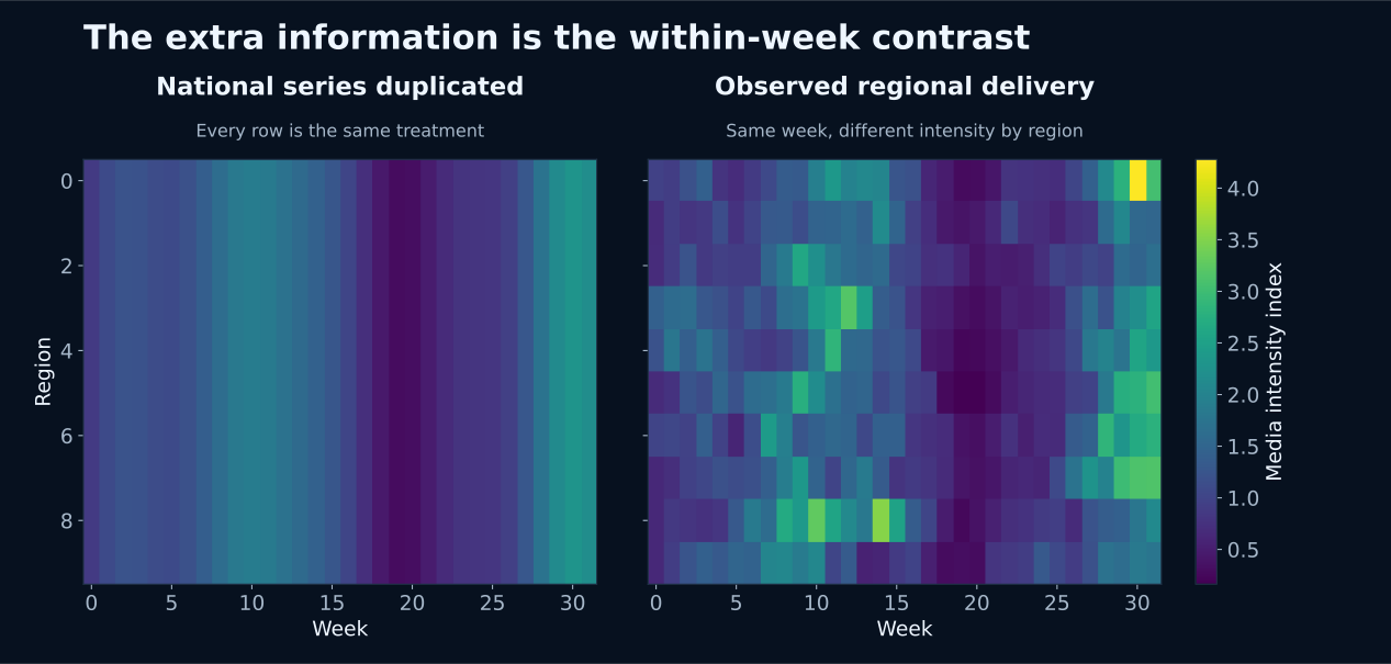
The interesting part is what remains of media after removing what is simply a region effect and what is simply a national time effect. For a linear illustration, define the two-way residualised treatment:
That object asks a useful question: did region g receive unusually high or low media at time t, relative to both its normal level and the national level that week? If the answer is yes, geography has supplied a treatment contrast.
If every region gets the same national series, so xg,t = Xt, then:
for every region and every week. The regional panel may still have plenty of variation in sales. It may have different intercepts, local weather, prices and distribution. But after allowing for the national time pattern, there is no regional media variation left to learn from.
A Bayesian way to see the same problem
Suppose, only for illustration, that after residualising the regional and time effects we fit:
with known noise σ. The posterior precision for β is:
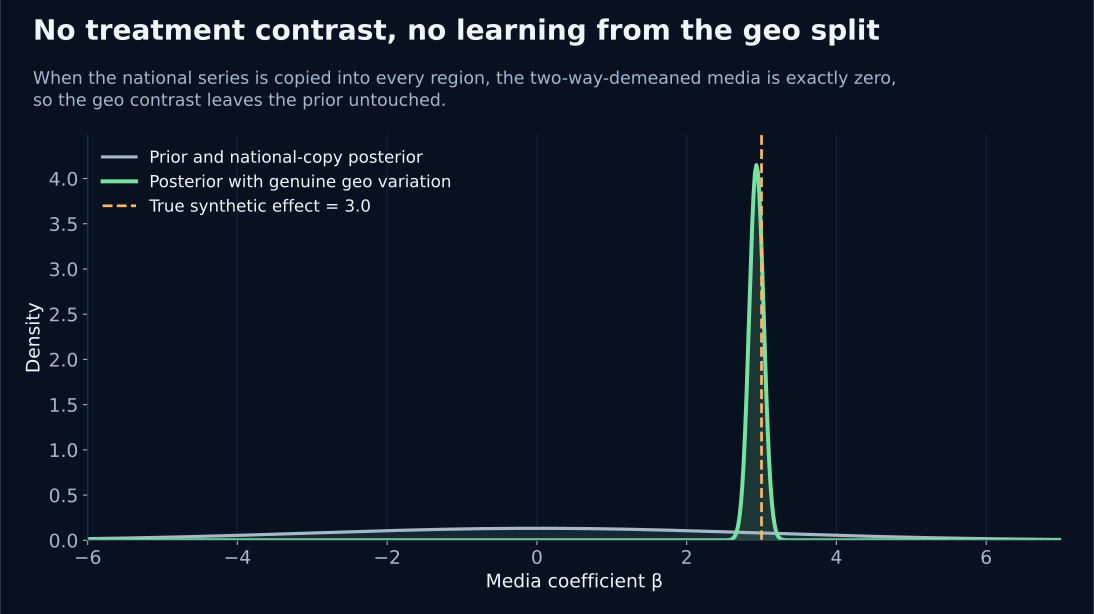
The second term is the information contributed by the treatment data. If the national media series is copied into every region, x̃g,t = 0, so that second term is zero. The geo contrast does not update the prior at all.
That is the cleanest way to state the issue. A hierarchy can shrink. A prior can regularise. More regions can help estimate regional baselines. None of those operations manufactures treatment variation that is not in the data.
A synthetic example: same row count, completely different information
We simulated 20 regions over 104 weeks. The national campaign plan moves over time, and there is also a national demand shock deliberately correlated with that plan. The true synthetic media coefficient is β = 3.0.
In the first version, actual regional delivery varies around the national plan, so regions receive different media intensity in the same week. In the second version, the national media series is simply duplicated across all 20 regions. Using a Normal prior β ~ Normal(0, 3²) and the two-way regional treatment contrast:
- with genuine geo variation, the posterior mean is 2.93, with an illustrative 95% interval of [2.74, 3.12];
- with the copied national series, the maximum absolute residualised treatment is about 1.1 × 10⁻¹⁵, numerical zero;
- therefore the copied-national posterior for the geo contrast is exactly the prior.
These numbers come from the reproducible synthetic example behind the figures. They are not empirical benchmarks.
There is an important caveat here. This does not mean a national MMM cannot estimate national media. A national time-series MMM can still use changes in Xt over time, together with controls, media transformations, priors, experiments and structural assumptions. The point is narrower: splitting the outcome into regions does not magically create an additional cross-sectional identification strategy for a treatment that is still national.
If you add a very flexible national time effect λt, the national media series is fully absorbed by it. If instead you use a more structured trend, seasonality and controls, the media coefficient can be estimated from time variation, but that is the same basic source of identification the national model had already.
Population apportionment is not regional media
A common workaround is to take national spend and allocate it to regions by population:
where sg is region g’s share of national population. The resulting spreadsheet now has a different spend number for every region. It looks like a geo media variable. But nothing happened in the real world. If population is Ng, then the invented spend per person is:
which is the same for every region. The regional difference disappears as soon as you remove the scale factor that created it.
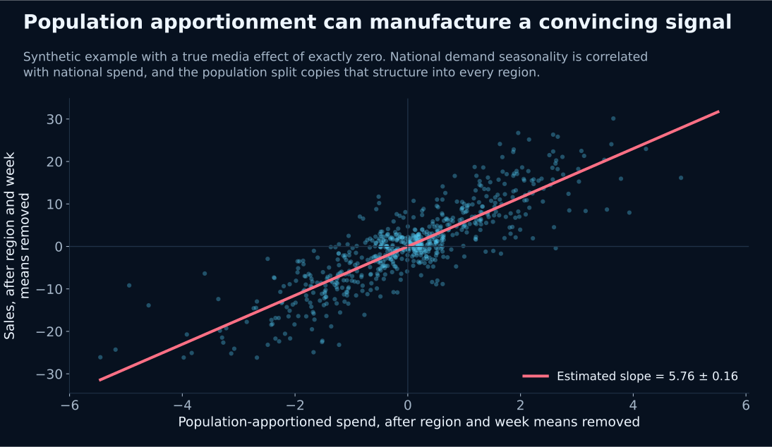
This matters because modelling totals can make the hack look surprisingly persuasive. Big regions naturally have more sales. A population allocation also assigns them more “spend”. If national demand conditions move with national campaign timing, the product of regional scale and national time movement can create a strong relationship even when the true causal media effect is zero.
We simulated exactly that case. The synthetic true media effect was set to zero. National spend and national baseline demand were correlated through seasonality, and national spend was then allocated to 18 regions by population share. The fake regional spend produced:
- a raw spend-to-sales correlation of 0.835;
- a two-way residualised slope of 5.76, with an approximate 95% interval of [5.60, 5.92];
- yet the true media effect was 0;
- and the within-week standard deviation of population-normalised allocated exposure was effectively 0.
Again, these are synthetic values in arbitrary units. Their purpose is to show how an accounting allocation can create false confidence, not to claim a universal bias magnitude.
Population can be a denominator without being an allocator
Population is often useful. The mistake is using it to pretend that national spend was geographically observed. Good uses include:
- scaling impressions or outcomes to a meaningful opportunity base;
- constructing per-capita or per-household measures;
- defining exposure rates against targetable population;
- setting known scaling constants in a panel model.
Those operations change units. They do not claim to know where the national budget was delivered. PyMC-Marketing’s multidimensional MMM supports additional panel dimensions through dims, including geography, with full, partial or no pooling across regions. Those are modelling and scaling capabilities, not evidence that a national spend series can be turned into observed geo treatment by allocation.
A national buy does not always mean identical regional treatment
This is the most important edge case. A campaign may be bought nationally but delivered unevenly. Digital auctions can produce different impressions, reach, frequency or CPM by region. Television delivery can vary with audience composition and inventory. Retail media may have different regional availability. A national campaign can therefore create genuine geographic exposure variation even if nobody set a separate regional budget.
If you have reliable region-by-time measures of realised exposure, that is not population apportionment. It is observed treatment variation. A geo MMM may then be useful.
However, variation alone is not automatically causal. Platform algorithms may deliver more media where predicted demand is already higher. Local inventory may respond to market conditions. Strong regions may receive more impressions because they generate cheaper conversions. Those mechanisms create targeting endogeneity: the geo model now has treatment variation, but you still need a causal story for why that variation is informative after controls, priors and calibration.
This is also why geo experiments are so powerful. Google’s original geo experiment framework assigns non-overlapping regions to different advertising conditions and implements the assignment through geo-targeted advertising. The variation is designed, not merely observed. Vaver & Koehler, 2011, Google Research
Measure the geo-identifying variation before you model
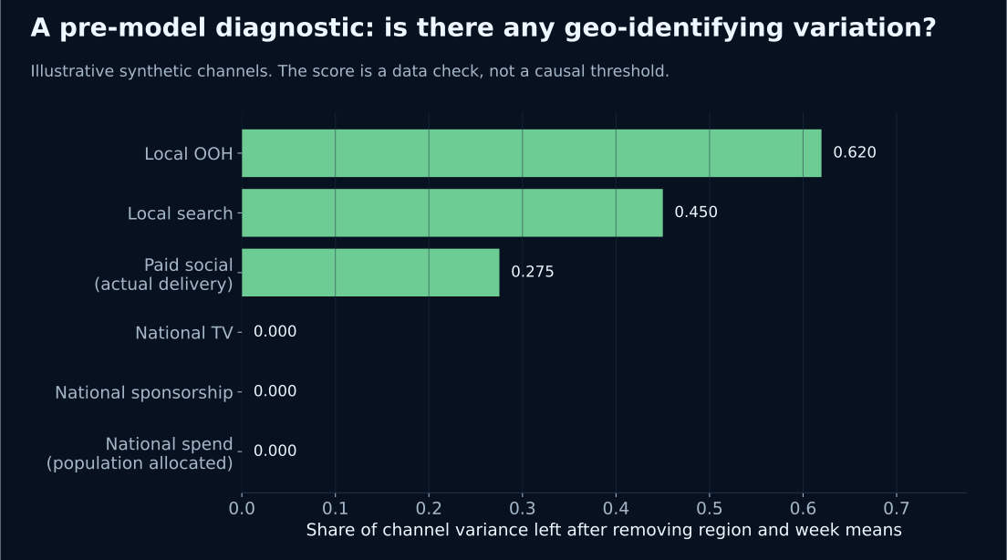
Before building a hierarchy, calculate how much channel variation survives after removing persistent region differences and common week differences. For each channel m, after first putting exposure on a sensible opportunity scale such as per targetable person, define:
where x̃ is the two-way residualised exposure from earlier. If Gm ≈ 0, almost all variation is regional scale or a common national time series. Larger values mean there is more region-by-time interaction for the model to exploit.
This is a diagnostic, not a causal score. A high value does not prove exogeneity, and there is no universal threshold. It simply answers the first question correctly: is there any geographic treatment contrast here at all?
A minimal implementation is two lines of NumPy:
# x has shape: region x date
x_tilde = (
    x
    - x.mean(axis=1, keepdims=True)   # remove region mean
    - x.mean(axis=0, keepdims=True)   # remove week mean
    + x.mean()
)

geo_variation_share = x_tilde.var() / x.var()
For a nonlinear MMM, run this first on the underlying exposure measure as a data diagnostic. You can also inspect the transformed media after adstock and saturation, but the conclusion will not change in the degenerate case: if every region starts from the identical series and uses the identical transformation, the transformed series remains identical.
From diagnostic score to expected precision
The diagnostic also gives you a rough sense of what the geo contrast is worth before you fit anything. From the conjugate result above, the data term in the posterior precision is Σ x̃² / σ², so for a panel with G regions, T periods and channel variance Var(x):
Holding the panel size, the noise level and the overall channel variance fixed, the credible interval width from the cross-sectional contrast scales with 1 / √Gm:
| Geo variation share | Interval width vs a fully geo-identifying channel |
|---|---|
| 0.01 | about 10× wider |
| 0.05 | about 4.5× wider |
| 0.10 | about 3.2× wider |
| 0.25 | about 2× wider |
| 0.50 | about 1.4× wider |
In the synthetic example above, the genuine-delivery panel had Gm ≈ 0.36, and 2,080 region-weeks were enough to shrink a prior standard deviation of 3.0 down to a posterior standard deviation of about 0.10. The same panel with the national series copied everywhere had Gm = 0: the formula collapses, and no amount of rows rescues it. The square-root scaling also cuts the other way: a channel with only a few percent of its variance in the region-by-time interaction needs a very large panel before the geo contrast tells you much, so a low score is a budget warning even when it is not exactly zero.
When is a regional MMM actually worth building?
A useful geo MMM usually passes most of the following tests.
- 1. Treatment varies within time. At the same week, month or day, regions receive meaningfully different media intensity. This can come from local budgets, local OOH, regional TV, search auctions, retail media, uneven digital delivery, rollouts or experiments.
- 2. The variation is measured, not invented. Use observed spend, impressions, reach, GRPs, insertions or another defensible exposure measure. Do not create treatment variation by multiplying a national total by population, sales share or historical market size.
- 3. The outcome is available at the same grain. Regional sales, leads or conversions need to align to the media geography and time grain. A mismatch in geographic boundaries can erase the advantage.
- 4. Important confounders are also regional. Price, distribution, promotions, availability, weather, competitor activity and local events can differ by geography. If those drivers are only observed nationally, a granular media file does not automatically solve confounding.
- 5. There is support, not just variation. If one region is always high-spend and another is always low-spend, media intensity may be inseparable from persistent regional characteristics. Useful designs contain enough overlap and movement to compare like with like.
- 6. Spillovers are limited or modelled. People cross borders. Media markets overlap. National creative can influence nearby geographies. A region is not automatically a sealed experimental unit.
- 7. The hierarchy is doing regularisation, not pretending to identify. Partial pooling is valuable when region-specific parameters are noisy. But pooling cannot substitute for treatment support. A hierarchical prior can stabilise an effect estimate; it cannot make an unobserved counterfactual suddenly observed.
The hybrid case is usually the real one
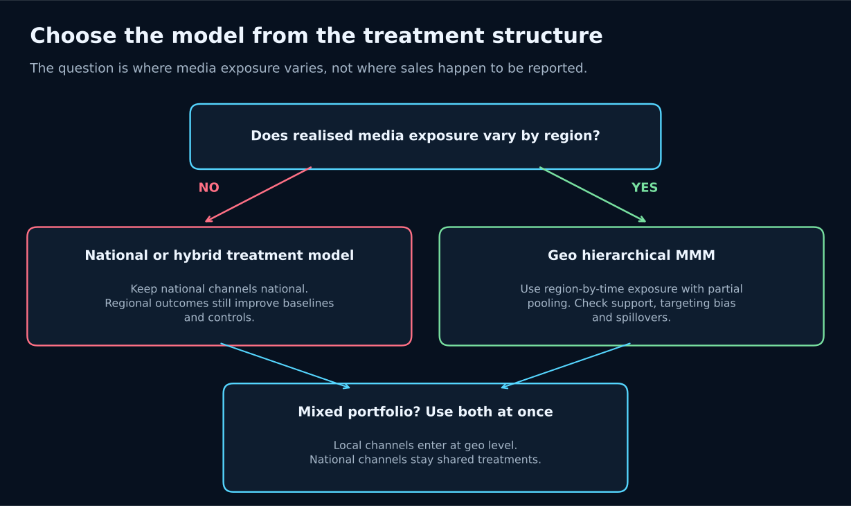
Most businesses do not have a perfectly national or perfectly local media plan. You might have national TV and sponsorship, locally delivered search and paid social, regional OOH, store-level promotions, national brand events, and local distribution and price. The right architecture is therefore often hybrid:
where L contains media with genuine local treatment and N contains national treatments shared across regions. That specification is honest about where the information comes from. Local channels use within-time geographic contrast. National channels are still identified from their national time movement, assumptions, controls, priors and calibration. Regional outcomes still contribute to the baseline and control structure without pretending that every media channel has become regional.
What this does not mean
It does not mean geo models are only useful for experiments. Observational regional media variation can be useful, provided the measurement and causal assumptions are credible.
It does not mean regional outcomes are useless when media is national. They can improve descriptive analysis, forecast local demand, model price and distribution, expose regional anomalies and support operational decisions.
It does not mean more rows never improve precision. Repeated regional outcomes can improve estimation of shared structures under appropriate error assumptions. The narrower claim is that identical media treatment does not create a new cross-sectional causal contrast for that media channel.
It does not mean a national buy always produces identical exposure. Measure realised delivery if you have it. The label on the buying process matters less than the treatment people actually received.
It does not mean a high geo-variation score proves causality. Variation is necessary for the cross-sectional argument, not sufficient. Targeting, omitted variables, spillovers and measurement error still matter.
The practical rule
Before anyone says “we can break sales out by region, so we should build a geo MMM”, ask one question: what media treatment actually differs across those regions at the same point in time?
If the answer is “none”, the geo split has not solved the media identification problem. Keep the national treatment national, and use the regional outcome where it genuinely adds information. If the answer is “we have real regional delivery variation”, then a hierarchical geo MMM can be a major upgrade. That is exactly the setting where more observations and useful variation can tighten estimates and help separate local media from shared national shocks.
The memorable version is simple: a geography column is not an identification strategy.
The industry tooling reflects the same logic. Google’s Meridian is built around geo-level data precisely because it carries more statistical information, and PyMC-Marketing’s multidimensional MMM gives you the same hierarchy with inspectable priors and pooling choices; we compared the two in PyMC-Marketing vs Google Meridian. In both cases the modelling decision should come before the software decision: use geography when the treatment, not just the reporting, is genuinely geographic.
Reproducibility note: all numerical examples and figures in this article come from deterministic synthetic simulations with fixed seeds. The simulations are intentionally simple, so the identification argument is inspectable rather than hidden inside a large MMM.
References
SIMBA is built on PyMC-Marketing, so geographic structure is a modelling choice you can inspect, not a default you inherit: national channels can stay national while local channels use the geo contrast they actually have. If you are weighing up a regional rebuild of your MMM, book a call and bring the diagnostic from this post.