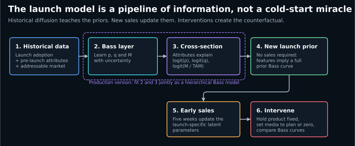
The fast answer: a new product has zero sales history, not zero information. Fit Bass curves to your completed launches, learn how pre-launch attributes predict p, q and M, and use that as the prior for the next launch. Update it as the first weeks of sales land. If you also make media an explicit intervention rather than just another correlated feature, the same structure gives you a do(media = 0) counterfactual curve.
A Bass diffusion model looks tailor-made for new products. It describes adoption from launch through acceleration and saturation, with an innovation parameter p, an imitation parameter q, and a market potential M.
There is still an awkward question: what do you put into the model before the new product has any sales?
A vague answer is "use priors from similar launches". A much more useful answer is to model what made those launches similar in the first place.
Build a database of historical launches. Estimate how pre-launch information predicts p, q and M. Then, for a completely new launch, turn its known launch plan and product characteristics into a probability distribution over the whole Bass curve. As sales arrive, update it.
And if media is modelled as an intervention rather than merely another correlated launch feature, you can generate a second Bass curve under do(media = 0) and estimate the launch sales that would plausibly have occurred without the media plan.
p captures external influence in the Bass mechanism. Causal media lift requires an explicit intervention model plus credible identification.What a Bass diffusion model is
Frank Bass published the model in 1969 to describe how new consumer durables spread through a market. It has survived because it captures, with only three parameters, the shape that first-time adoption keeps taking in practice: a launch, an acceleration as the product becomes social, a peak, and a long tail as the market saturates.
The mechanism is two pressures acting on everyone who has not yet adopted. External influence (advertising, press, shelf presence) reaches people whether or not anyone else has adopted. Internal influence (word of mouth, imitation, visible use) grows with the installed base. Bass wrote the chance that an eligible non-adopter adopts right now as:
where F(t) is the fraction of the eventual market that has already adopted. On day one F = 0, so only the external pressure p is working; as adoption builds, the social term q F(t) takes over. Integrating the hazard gives the familiar closed forms. The cumulative adoption fraction is:
and the new-adopter rate is:
so expected new adopters at time t are M f(t), and cumulative adoption tends towards M.
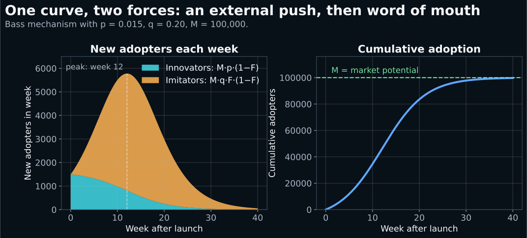
That picture is the whole vocabulary of the model:
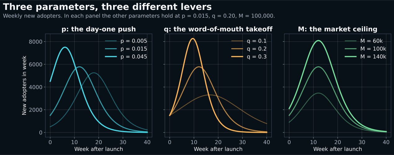
p: innovation, or external influence. It helps adoption get moving before many other adopters exist.q: imitation, or internal influence. It governs how strongly adoption accelerates as the installed base grows.M: market potential. It controls the eventual adoption ceiling.
Two of the levers interact in a way worth knowing by heart. When q is larger than p, the adoption peak lands at t* = ln(q/p) / (p + q), so strengthening word of mouth does not just raise the peak, it pulls it forward. The parameters also have folklore magnitudes: the classic meta-analysis of annual durable-goods applications found typical values near p ≈ 0.03 and q ≈ 0.38. On the weekly grid used later in this article, the same mechanism simply lives at different scales.
None of this needs bespoke code any more. PyMC-Marketing ships a BassModel that takes single-product and multi-product data, accepts configurable priors for m, p, q and the likelihood, and exposes posterior deterministics including adopters, innovators, imitators and peak. The official notebook demonstrates Bayesian fitting across several products at once.
But these three parameters are exactly why a genuinely new launch is hard. A new product has no sales history from which to identify them.
The trick is not to make Bass magically identify them from nothing. It is to learn a prior model for those parameters from previous launches.
Build a launch database, not a library of arbitrary analogues
There is useful precedent for this idea. Lenk and Rao were using hierarchical Bayes for early new-product forecasting in 1990, explicitly allowing older products to inform a new launch and then letting the new launch adapt as its own sales arrived. A 2014 paper by Lee and colleagues went further in a cross-sectional direction: it built product-attribute and diffusion databases for 87 products, then predicted Bass parameters before launch using regression and machine-learning methods.
The modern Bayesian version can combine both ideas. Instead of choosing one analogue, or treating fitted Bass parameters as perfect labels, we can estimate a distribution of launch-level p, q and M, explain their variation using launch features, and carry all that uncertainty into the next product.
A useful launch table can be much richer than "category" and "brand". For example:
| Feature family | Examples known before launch | Why it might matter |
|---|---|---|
| Product | Price premium, generation change, feature novelty, form factor, compatibility, replacement cycle | Can change adoption friction, differentiation and reachable demand |
| Brand | Awareness, consideration, brand strength, installed base, historical category strength | Can move initial willingness to adopt and total potential |
| Demand signals | Pre-launch search, waitlist size, pre-orders, landing-page traffic, email sign-ups | Early evidence of latent demand before sales exist |
| Distribution | Planned doors, weighted distribution, countries, launch-day availability, inventory cover | Controls who can actually buy, and how quickly |
| Paid media | Pre-launch spend, committed launch-window spend, expected reach, frequency, channel mix, share of voice | Can affect external adoption and, depending on the causal structure, effective reach |
| Launch events | Keynote, livestream, press event, reviewer embargo, creator seeding, PR commitment | Can create a concentrated external shock around launch |
| Commercial plan | Introductory price, bundles, trade-in, retailer media, promotional depth | Changes adoption economics and visibility |
| Market context | Category growth, penetration headroom, season, competitor launch proximity, competitor share of voice, macro conditions | Helps separate the product from the environment it launched into |
The leakage rule matters. If the forecast is made before launch, the feature set should only contain information that genuinely existed at that point. Realised review scores, achieved organic PR, realised distribution and post-launch search are not harmless predictors. They can be future information, or mediators of the treatment you later want to evaluate.
The cross-sectional model on p, q and M
For launch i, let Xi contain standardised pre-launch features. In the worked example we transform the Bass parameters and regress them on those launch features:
For the synthetic example, zp = logit(p), zq = logit(q), and zM = logit(M / A), where A is an externally supplied addressable market. That last transformation guarantees that fitted M cannot exceed the stated addressable population.
The logit choice for p and q is convenient here because we deliberately simulate a practical weekly parameter domain inside (0, 1). It is not a universal Bass requirement. If your time scale permits larger q, use a positive unbounded link such as log(q) instead.
A stronger production model would make (upi, uqi, uMi) multivariate with an LKJ prior on their residual correlation. That lets the hierarchy learn, for example, that launches with unexpectedly high innovation also tend to have unexpectedly high market potential, even after accounting for observed features.
Yes, this should really be a hierarchical Bass model
There are two ways to implement the idea.
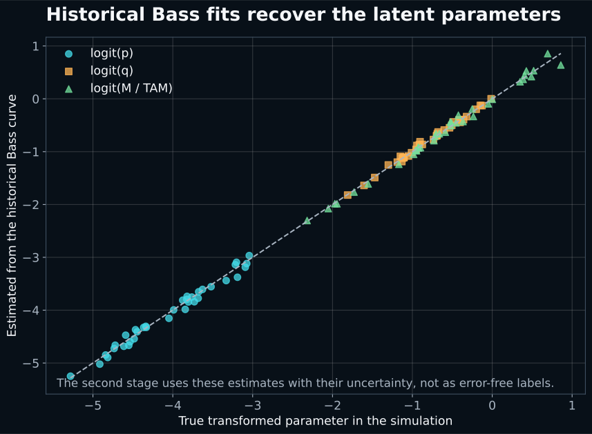
Two-stage version: fit a Bass curve to each completed launch, obtain uncertain estimates of pi, qi and Mi, then fit Bayesian measurement-error regressions of those parameters on launch features. This is modular, quick to debug and easy to explain.
Joint hierarchical version: keep every launch-specific Bass parameter latent and fit the cross-sectional relationships and all historical sales curves in one model:
The second version is the one I would want in production. It avoids pretending that the first-stage parameter estimates are data observed without error, it naturally pools weak launches more strongly, and it learns the launch-feature relationships at the same time as the diffusion curves.
For this article, the executed example uses the two-stage approximation with explicit first-stage uncertainty, because it keeps the computational demonstration compact.
A worked launch portfolio, actually sampled
We simulated 36 historical launches, each with 48 weeks of adoption and an externally supplied addressable market. Each launch had six features: brand strength, pre-launch search, planned day-one distribution, a keynote indicator, launch media spend, and price premium.
The data-generating process deliberately made different features affect different parts of diffusion. Launch media was strongly related to p, only weakly related to q, and moderately related to effective market potential. Distribution mostly affected M. Keynotes mostly moved p. Price premium reduced both external adoption and market potential.
We then fitted three Bayesian cross-sectional measurement-error models in PyMC. These were genuine NUTS samples, not hand-drawn uncertainty bands. Each posterior contained 1,400 draws across two chains after tuning, and the maximum split-chain R-hat across the cross-sectional parameters was 1.002.
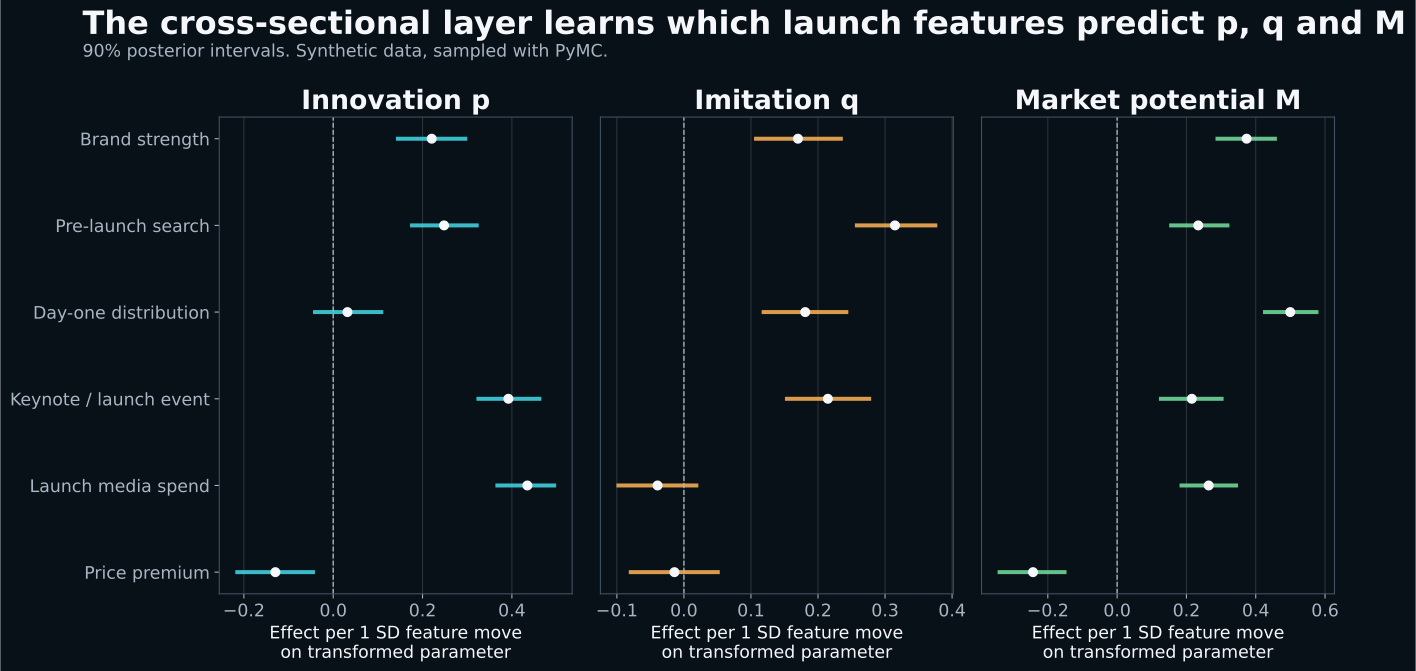
This is the part that makes a true cold-start forecast possible. For a new launch with no adoption history, plug its known features into the cross-sectional posterior. Every posterior draw produces a plausible p, q and M, which produces a plausible Bass curve.
Forecast the launch before the first sale
Our unseen synthetic launch had strong pre-launch search, strong brand strength, high planned distribution, a keynote, 145k of launch media in the synthetic budget scale, a small price premium, and an addressable market of 260,000.
Before using a single sale from the new product, the historical launch model already produces a distribution of adoption curves.
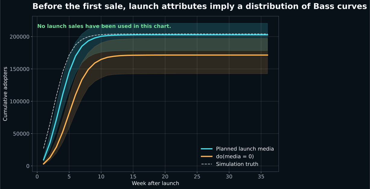
This is much better than dropping a generic p = 0.02, q = 0.4 prior into every launch. It says that an established brand with large pre-launch demand signals, high availability and a keynote should not start with the same prior as an obscure product entering a weak category with limited distribution.
It also gives the forecast a useful decomposition. We can ask whether uncertainty is mostly about the launch ceiling M, the initial external push p, or the strength of imitation q. Those imply different business actions.
Then let the new launch become itself
The population model should not dominate forever. Once the first weeks of launch sales arrive, the launch-specific likelihood updates the feature-informed prior.
In the worked example we expose the model to only the first five weeks of observed adoption. The causal launch model is then sampled again with PyMC, and the maximum R-hat across its key latent parameters is 1.0003.
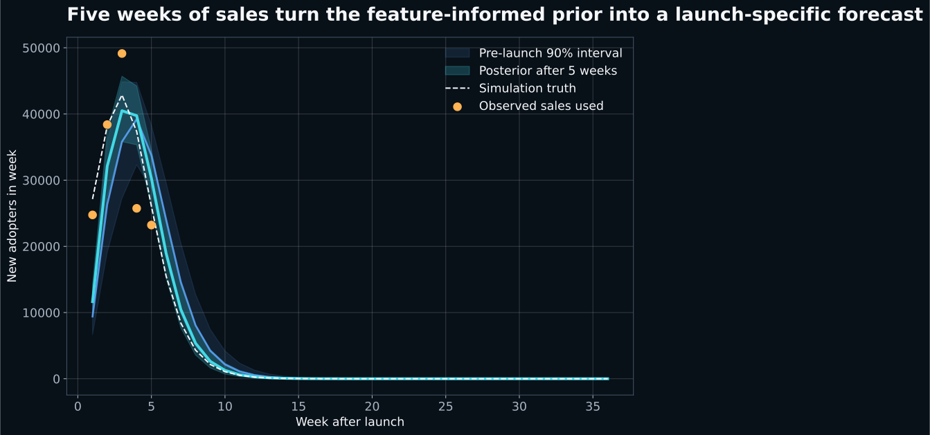
This is the original hierarchical Bayes promise in a modern form: borrow strength when the launch is data-poor, then relinquish it as the launch becomes data-rich.
Now make media a causal intervention
This is where we need to be stricter than a standard Bass interpretation.
PyMC-Marketing describes p as external influence, and its innovator component can include advertising or mass media. That does not mean that a fitted p is automatically a causal advertising effect. A product can have a high p because it is inherently newsworthy, because the brand is famous, because it launched into unusually strong demand, or because management anticipated a blockbuster and funded it heavily.
To measure media, make the media plan an explicit intervention in the parameter model. Split each transformed parameter into a no-media baseline plus a media pathway:
where η contains the product, the brand, the market context and the launch-specific residual, and a is the media intervention.
For each posterior draw, calculate two potential outcomes while holding the same product and latent residual fixed:
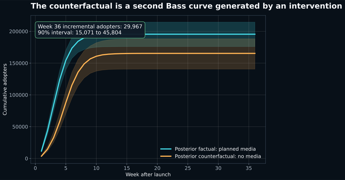
S0(t) is the counterfactual Bass curve under do(media = 0). This is exactly the question we wanted: if this same product had launched into the same market without the planned media, how would its diffusion path have changed?
In our sampled synthetic example, the posterior median at week 36 is about 195,479 cumulative adopters with the media plan and 165,330 without it, giving 29,967 incremental adopters. The 90% posterior interval for incremental adoption is roughly 15,071 to 45,804. The simulation truth was 29,149, so the deliberately identifiable toy model lands in the right area.
There is historical precedent for putting marketing decision variables into diffusion, rather than treating the plain Bass curve as the whole causal story. Bass, Krishnan and Jain's 1994 Generalized Bass paper explicitly extended the model to include decision variables such as advertising and price.
Should media change M as well as p?
Sometimes. But that choice changes the estimand, so it needs to be explicit.
If M means a physical addressable market, such as every eligible customer who could realistically buy the product, then media should probably not change it. Media changes the rate at which that market adopts, perhaps mainly through p, while the ceiling remains fixed.
If M means an effective reachable market potential, then media can plausibly move it. Awareness can bring more of the nominal market into the eventual adopter pool. In that model, the no-media Bass curve can have both a slower start and a lower ceiling.
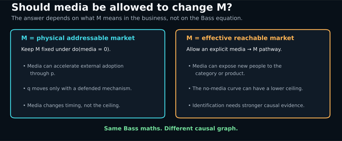
I would normally report at least two scenarios: a conservative timing-only media effect with M fixed, and an effective-market specification where media can move M, supported by stronger evidence. If the business decision changes materially between them, that is useful sensitivity, not an inconvenience to suppress.
The hard part is identification, not sampling
The synthetic example is intentionally friendly: historical launch media is assigned independently enough that the media coefficient is identifiable from the launch database. Real launch budgets are rarely like that.
Management spends more on launches it expects to succeed. Big brands get more distribution and bigger keynote events. Products with strong pre-orders may receive extra launch investment. Competitor activity can change both budget and sales. A Bayesian posterior does not remove those paths.
So separate two jobs:
- Prediction of
p,qandM. Throwing in useful pre-launch predictors can be entirely reasonable if the goal is forecasting. - Causal effect of media. The media coefficient needs a defensible causal design.
For the second job, useful evidence could include randomised geo or audience tests, historical budget shocks, instruments, quasi-experiments, explicitly modelled budget-setting variables, or experimental calibration priors on γp, γq and γM. If none of those is available, call the media pathway predictive association rather than causal lift.
A practical causal graph would also distinguish confounders from mediators. Planned distribution may confound the relationship between launch budget and demand if it affected both decisions before launch. Realised awareness after the campaign may be a mediator of media. Conditioning on the latter can block part of the effect you are trying to measure.
What if media varies week by week?
The scalar launch-media intervention above is deliberately simple. Many launches have a pre-launch teaser, a keynote spike, a launch burst and then a long tail of support.
For that case, extend the diffusion mechanism rather than compressing everything into one number. Two sensible approaches are:
- let the external adoption component vary over time, for example
pt = g(mediat, PRt, pricet, …), while retaining the imitation feedback through cumulative adoption; - use a Generalized Bass-style decision-variable component that speeds up or slows down diffusion as marketing inputs change.
The stock BassModel in PyMC-Marketing gives us an excellent base Bass implementation and configurable priors. A time-varying causal media mechanism is a custom extension in PyMC, rather than something to assume the class is doing automatically.
That custom extension is actually attractive, because it starts to connect diffusion forecasting with MMM. Media has carryover, saturation and channel-specific response. Bass supplies the adoption state. A causal media model supplies the intervention. The two do not need to be competing explanations. For the response side of that, see Bayesian MMM Explained.
A PyMC-Marketing implementation pattern
The current PyMC-Marketing API lets us pass custom priors into BassModel. So the feature model can generate prior draws for a new launch, moment-match or otherwise approximate those draws with supported prior families, and then let BassModel update from observed adoption.
from pymc_extras.prior import Prior, Scaled
from pymc_marketing.bass import BassModel

# p_prior, q_prior and m_share_prior come from the launch-feature model.
model = BassModel(
    model_config={
        "p": Prior("Beta", alpha=p_alpha, beta=p_beta),
        "q": Prior("Beta", alpha=q_alpha, beta=q_beta),
        "m": Scaled(
            Prior("Beta", alpha=m_alpha, beta=m_beta),
            factor=addressable_market,
        ),
        "likelihood": Prior("NegativeBinomial", n=40.0),
    }
)

idata = model.fit(data=first_five_weeks)
One reproducibility detail is worth being explicit about. The environment used to build this article contained PyMC 5.27.1 but not the PyMC-Marketing wheel, and could not install packages. The published synthetic posterior numbers were therefore sampled with PyMC directly, using the same Bass F and f equations that PyMC-Marketing documents and implements. Nothing in the numerical demonstration depends on a hidden closed-source implementation.
What I would build for a real launch portfolio
A production system would have four layers:
- 1. Historical launch hierarchy. Jointly fit weekly adoption across products, markets and launch cohorts. Partial pooling can exist at brand, category, geography or generation level where the data supports it.
- 2. Pre-launch parameter model. Let known launch attributes shift the population distribution of
p,qandM. Include a residual covariance structure rather than three unrelated regressions where possible. - 3. Causal treatment layer. Treat media, launch event intensity, price or distribution interventions separately from ordinary predictors. Put experimental evidence directly into priors for treatment pathways.
- 4. Sequential update. Before launch, forecast entirely from the hierarchy. After week one, week two and week five, update the launch-specific posterior. Watch for the new product systematically escaping the historical population, which is information in itself.
There are useful extensions beyond that. A global product company could use a multi-level hierarchy such as product generation within brand within category, with market-level variation layered on top. A staggered international launch could share a global product latent effect while allowing country-specific distribution, price and media to alter diffusion. A portfolio planner could then simulate counterfactual launch calendars and media plans before committing inventory.
What this does not mean
Bass is not a universal sales curve. It is most natural when the outcome represents adoption of a product or service by new units over time. Repeat purchases, stockpiling, churn, supply constraints, subscriptions with reactivation, and strong replacement cycles may require a richer state model.
The cross-sectional hierarchy also does not create information out of nothing. If you have only four historical launches and twenty highly correlated launch features, the feature coefficients should remain broad. Strong shrinkage and simpler group-level pooling will usually beat an elaborate launch "AI score".
Most importantly, forecasting and causality are different layers. A feature can be an excellent predictor of M while being useless as a causal lever. A launch-media coefficient can be highly precise and still be biased if budget allocation is endogenous.
The takeaway
A new product can have zero sales history without having zero information.
Use completed launches to learn a population distribution for Bass p, q and M. Let pre-launch product, brand, demand, distribution and marketing features shift that distribution. Fit the structure hierarchically so uncertain launches borrow strength. Then update with the new product's own sales as soon as they arrive.
For media effectiveness, go one step further. Make media an intervention in the generative model and compare the factual Bass trajectory with a posterior do(media = 0) trajectory. That gives you a counterfactual curve, not just a story about a high innovation coefficient.
Bass forecasts the curve. The hierarchy solves the cold start. The causal layer tells you what the launch plan actually changed.
The worked example in this article is synthetic, and deliberately so: simulating the data is what makes the true causal effect knowable, so the recovered interval can be checked against it. It is evidence that the modelling workflow behaves coherently, not empirical evidence that any particular real launch would receive the same media effect.
References
BassModel API. pymc-marketing.io/…/BassModelSIMBA is built on PyMC-Marketing, so the priors, the pooling and the counterfactual are all inspectable rather than hidden behind a single launch forecast number. If you have a portfolio of completed launches and a new one coming, that history is worth more than a spreadsheet analogue. Book a call to talk through what your launch database could support.