The fast answer: do not ask an MMM to invent the value of a customer. If lifetime value is not trustworthy, optimise the allocation at a fixed spend level and compare it with the historical allocation. If value per incremental acquisition is trustworthy, put that value inside the objective. The optimiser can then decide both where to spend and how much to spend.
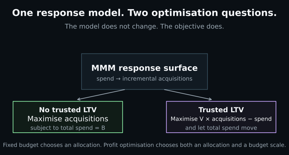
Marketing budget optimisation often gets framed as a choice between two different models: one that maximises conversions and another that maximises profit. That is usually the wrong mental model.
The hard statistical work is estimating the response to spend. Once the MMM has learnt how incremental acquisitions change as each channel moves through adstock and saturation, the optimisation problem sits on top of that response surface.
What changes is the objective.
If finance has already set a £200k budget, the question is straightforward: what allocation gets the most acquisitions from £200k? If the business also trusts that each incremental acquisition is worth, say, £50 in discounted contribution value, the question becomes different: what allocation and total spend maximise expected contribution value after marketing cost?
Those are not rival methods. The second problem contains the first.
Start with the response model, not the objective
Write the expected incremental acquisitions over the planning horizon as:
where s is the vector of channel spends. The model can be arbitrarily realistic: adstock, saturation, geo dimensions, channel interactions, time-varying effects and posterior uncertainty can all sit inside A(s).
For the worked example below, we deliberately use something simpler so the mechanism is visible. Each channel has a saturating response:
The values are illustrative, not client data. Spend is measured in £000 and acquisitions in 000s.
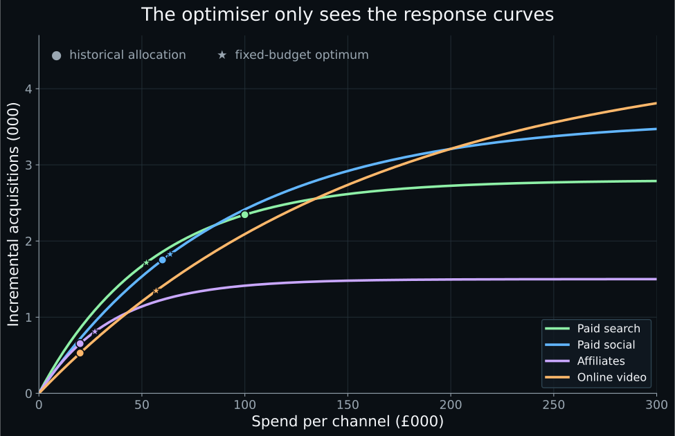
The curves already contain the key economic fact: the next £1,000 does not generate the same number of acquisitions everywhere. As a channel saturates, its marginal response falls.
That is what the optimiser exploits.
Mode 1: no trusted LTV, so maximise acquisitions at fixed spend
Suppose total marketing spend has already been decided as B. Then the objective is:
plus whatever practical channel bounds and business rules apply.
This is the safest formulation when you trust the MMM response but do not trust the conversion-to-value layer. You are not pretending that a new customer is worth £80, £120 or £250. You are simply asking for the best allocation of a budget that has been set elsewhere.
The correct benchmark is the historical allocation at the same total spend. That matters because otherwise the optimiser gets credit for changing both efficiency and scale.
In our toy example the historical £200k allocation is:
| Channel | Historical | Max acquisitions at £200k |
|---|---|---|
| Paid search | £100k | £52k |
| Paid social | £60k | £64k |
| Affiliates | £20k | £27k |
| Online video | £20k | £57k |
| Total | £200k | £200k |
The historical mix produces about 5.28k incremental acquisitions. Reallocation on the same response curves produces about 5.70k, an illustrative uplift of 8.0% with no extra money.
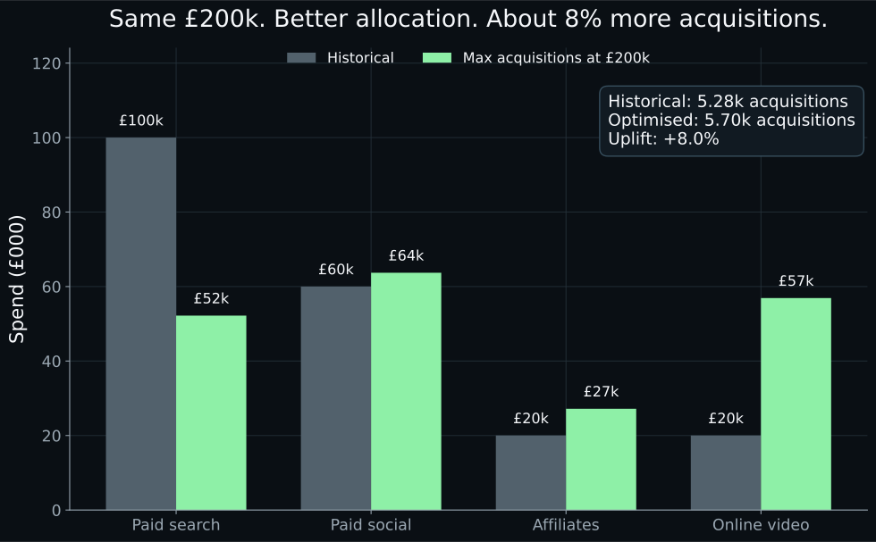
At an interior optimum, the active channels are pushed towards the same marginal acquisitions per pound. If one channel could still generate materially more acquisitions from the next pound than another, shifting money towards it would improve the objective.
That is the fixed-budget condition. It says nothing about whether £200k itself is too high or too low.
Mode 2: trusted LTV, so maximise value minus spend
Now suppose the business has a defensible value V for each incremental acquisition. The objective becomes:
There is no economic reason to force Σsᵢ to equal the old budget. Spend is now a decision variable.
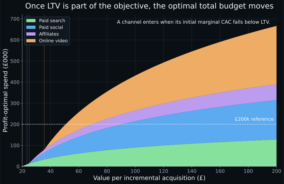
This is the crucial difference. If an incremental acquisition is worth more, the model should be willing to buy deeper into the response curves. If it is worth less, the model should stop earlier.
The two modes are easier to see if we define the efficient acquisition frontier:
F(B) answers the fixed-budget question for every possible budget level. Profit optimisation is then just:
So the profit problem is not a new response model. It is the same fixed-budget frontier with one additional choice: which point on the frontier is economically worth buying?
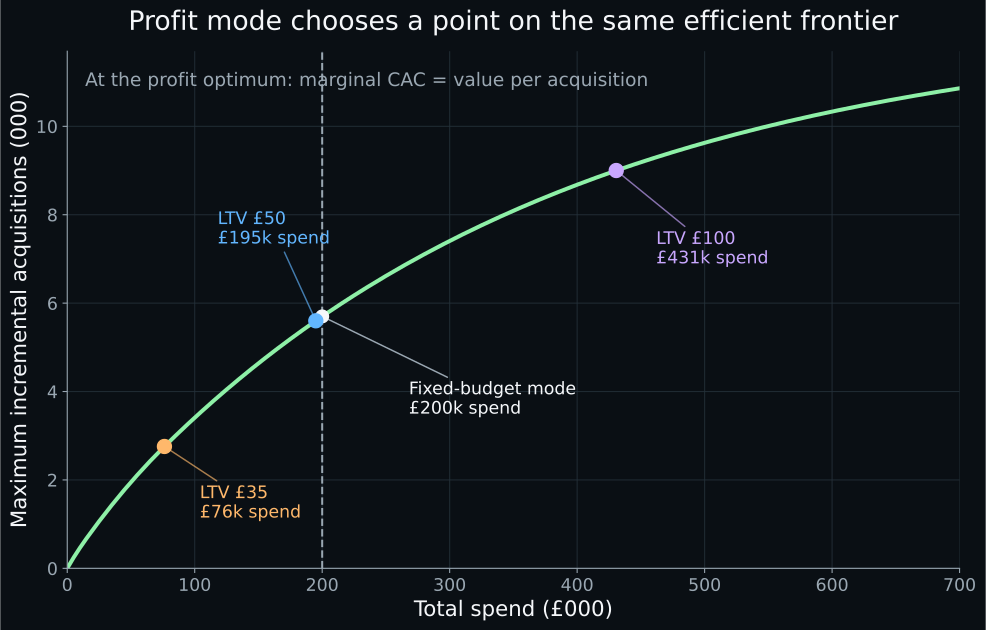
In this simulation:
| Objective | Total spend | Incremental acquisitions | Expected marketing profit |
|---|---|---|---|
| Max acquisitions, fixed budget | £200k | 5.70k | not defined without value |
| Max profit, V = £35 | £76k | 2.76k | £20k |
| Max profit, V = £50 | £195k | 5.60k | £85k |
| Max profit, V = £100 | £431k | 9.00k | £469k |
Illustrative profit here means V × incremental acquisitions − marketing spend. In a real implementation, V should already be the appropriate net contribution value for the outcome being optimised.
The response curves did not change between those rows. Only the value assumption changed.
The stopping rule is marginal CAC = LTV
The profit objective gives a very useful first-order condition. For an active channel at an interior optimum:
Rearranging:
This is the practical rule to remember.
The optimiser keeps spending until the next acquisition costs as much as that acquisition is worth. That is marginal CAC, not average CAC. A channel can have an average CAC comfortably below LTV while its next pound of spend is already uneconomic. Conversely, stopping whenever average CAC reaches LTV will generally stop too early, because the earlier, cheaper acquisitions are pulling the average down.
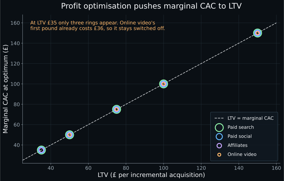
This also explains why total spend can move sharply with LTV.
What counts as a trusted LTV?
This is where most of the business judgement lives.
A value estimate does not need to be known with perfect precision before it is useful. It needs to be reliable enough that the budget recommendation is stable over the plausible range. If an LTV of £45 implies £160k of spend and £55 implies £235k, that sensitivity is decision-relevant. If every plausible value between £45 and £55 produces roughly the same plan, you do not need false decimal-point precision.
The bigger risk is using the wrong value concept entirely. For profit optimisation, V should usually be discounted incremental contribution value, not headline revenue LTV. If the model outcome is a lead rather than an acquired customer, then customer LTV cannot be multiplied directly by leads unless the lead-to-customer conversion and its economics are already incorporated. If acquired customers differ in quality by channel, market or cohort, a single scalar LTV can also distort allocation.
PyMC-Marketing’s CLV tools explicitly support discounted lifetime-value calculations, and its Gamma-Gamma workflow notes that monetary value can represent profit or revenue as long as it is defined consistently. That flexibility is useful, but the optimiser still needs the value concept that matches the business objective. See the CLV utility documentation and the CLV quickstart.
A good practical test is to ask five questions before switching to floating-spend profit mode:
- Does the value correspond to the exact outcome the MMM predicts?
- Is it contribution value rather than top-line revenue if the stated objective is profit?
- Are retention, fulfilment, servicing and discounting treated consistently?
- Does customer quality vary enough by channel or segment that one scalar value is misleading?
- Is the recommended budget reasonably stable across the credible LTV range?
If several of those answers are shaky, fixed-budget acquisition optimisation is not a second-rate fallback. It is the correctly scoped question.
The Bayesian version should propagate both uncertainties
An MMM does not really give one response curve. It gives a posterior distribution over response curves. LTV may also be uncertain.
The natural extension is therefore:
where θ represents MMM uncertainty and V can itself be a distribution. A more conservative business can replace expected profit with a risk-adjusted utility, for example penalising downside or optimising a lower-tail measure.
This is one place where the current PyMC-Marketing optimiser is structurally helpful. The BudgetOptimizer accepts a custom utility function, and that utility receives both posterior response samples and the candidate budgets. Its current source also makes the constraint behaviour explicit: with no custom constraints it adds a default sum(spend) = total_budget equality, while non-empty custom constraints put the caller in charge. That makes both modes natural implementations of the same optimiser.
Schematically, the profit utility is almost embarrassingly simple:
def expected_profit(samples, budgets, value_per_acquisition):
    expected_acquisitions = samples.mean()
    marketing_spend = budgets.sum()
    return value_per_acquisition * expected_acquisitions - marketing_spend
The important implementation change is not the formula. It is the constraint set. Fixed-budget mode uses an equality constraint. Floating-spend mode removes that equality and normally replaces it with sensible channel bounds and a total spend ceiling, so the optimiser does not extrapolate into regions the model has never learnt.
What this does not mean
Profit optimisation is only as credible as the response curves and the value layer it joins together.
It does not mean that an MMM can tell you your customer LTV. It does not make wild extrapolation beyond historical spend safe. It does not solve channel-specific customer-quality differences unless those are modelled. It does not mean every business should let an optimiser freely set the annual marketing budget. And it does not remove the need for constraints around inventory, reach, channel capacity, minimum commitments, brand floors or operating risk.
There is another subtlety. If the MMM estimates conversions that would have happened through another channel anyway, or if the conversion outcome is not truly incremental, then multiplying by LTV can make the profit objective look more precise than the causal estimate warrants. The economic layer cannot rescue a weak response model.
A simple decision rule
The historical allocation should still be shown in both cases. In fixed-budget mode it is the direct benchmark. In profit mode it is a useful reference point that shows whether the model is recommending a change in mix, a change in scale, or both.
The takeaway
The question is not “should my optimiser maximise conversions or profit?” as though those require two competing models.
Build one credible response model. Then choose the objective that matches the information the business actually trusts.
- No trusted LTV: maximise acquisitions subject to a spend constraint.
- Trusted LTV: maximise value times acquisitions minus spend, and allow total spend to move within sensible bounds.
The second mode is simply the first mode with an economic value attached to the frontier. That is a much cleaner way to connect MMM response curves to an actual budget decision.
The numerical example in this article is synthetic. Four channels follow A(s) = Amax(1 − exp(−s / k)) with spend in £000 and acquisitions in 000s. The fixed-budget allocation is solved with SLSQP, and the floating-spend optimum uses the closed form s* = max(0, k · log(V · Amax / k)) that falls out of the first-order condition. For what happens upstream of the optimiser, see Bayesian MMM Explained.
References
BudgetOptimizer documentation. pymc-marketing.io/…/BudgetOptimizerallocate_budget documentation. pymc-marketing.io/…/allocate_budgetBudgetOptimizer source on main. github.com/pymc-labs/pymc-marketingSIMBA uses PyMC-Marketing response models and budget optimisation to make these assumptions inspectable rather than hiding them behind a single “optimal budget” number. The most important input is not the solver, it is being explicit about what you are asking the solver to optimise. If you want to pressure-test which mode your plan should be in, book a call.