Marketing mix models often end with a deceptively simple chart: base sales at the bottom, channel contributions stacked on top, and fitted sales at the top. That picture is straightforward when the model is additive. It becomes much less obvious when the model is multiplicative.
If TV, Search and Social multiply the outcome rather than add fixed units to it, then asking “how many sales belong to TV?” is no longer answered directly by the model equation. Remove TV on its own and you get one number. Remove Search on its own and you get another. Add those removal effects together and they can exceed the total amount of incremental outcome that actually exists.
This is not a modelling bug. It is an attribution problem. In this post we will:
- build a tiny multiplicative MMM by hand;
- show why one-at-a-time channel removal double-counts outcome;
- compare the main ways to turn a multiplicative prediction into additive contributions;
- look at standard Shapley, permutation Shapley and Aumann-Shapley;
- test the methods as the number of model components grows from 2 to 40;
- stress-test the methods when positive and negative effects coexist.
The central point is simple: a multiplicative MMM identifies the fitted outcome, the reference outcome and the total incremental lift exactly. It does not, by itself, uniquely determine an additive channel-level decomposition of that lift. The contribution split requires an attribution rule: a convention for distributing the interaction created by multiplication. That rule is part of the reporting methodology, and it should be explicit.
One consequence of that framing runs through this whole post, so it is worth stating up front. When we compare decomposition methods later, we will be measuring two fundamentally different things. Approximation error arises when an algorithm is estimating a defined target (permutation Shapley estimating exact discrete Shapley) and can be driven down with more computation. Attribution-definition differences arise when two methods answer different counterfactual questions (Aumann-Shapley versus discrete Shapley) and no amount of computation removes them, because neither method is wrong. Keeping those two ideas separate is the main job of this article.
Start with the model
Consider a log-link multiplicative MMM:
μ = Base × exp(q₁ + q₂ + ⋯ + qₙ)Here, μ is the fitted outcome with all model components at their observed values. Each q is the log-scale effect for a player. In a real MMM that player could be:
- TV after adstock and saturation;
- Paid Search after its media transformation;
- Social;
- price;
- distribution;
- seasonality;
- a holiday effect;
- another control or event effect.
For media, q is not raw spend. It is the modelled log contribution after the media transformation chain. If we remove every player, the reference outcome is the base, and the total incremental outcome explained by the players is:
Base = μ × exp(−(q₁ + q₂ + ⋯ + qₙ))

L = μ − Base = μ × (1 − exp(−Σ q))
That total is not ambiguous. It is worth being precise about the division of labour here, because it is the source of everything that follows:
The model itself gives us:
  - the fitted outcome μ
  - the baseline / reference outcome
  - the log-scale effects q
  - the total joint incremental lift L

The decomposition method then determines:
  - how that total lift is divided between players
The difficult question is the second part: how to split L across the individual players.
A two-channel MMM
Take a deliberately small example: fitted outcome μ = 100, with q_TV = 0.5 and q_Search = 0.3. The implied baseline is 100 × exp(−0.8) = 44.93, and the media multipliers are exp(0.5) ≈ 1.649 and exp(0.3) ≈ 1.350. Together:
44.93 × 1.649 × 1.350 = 100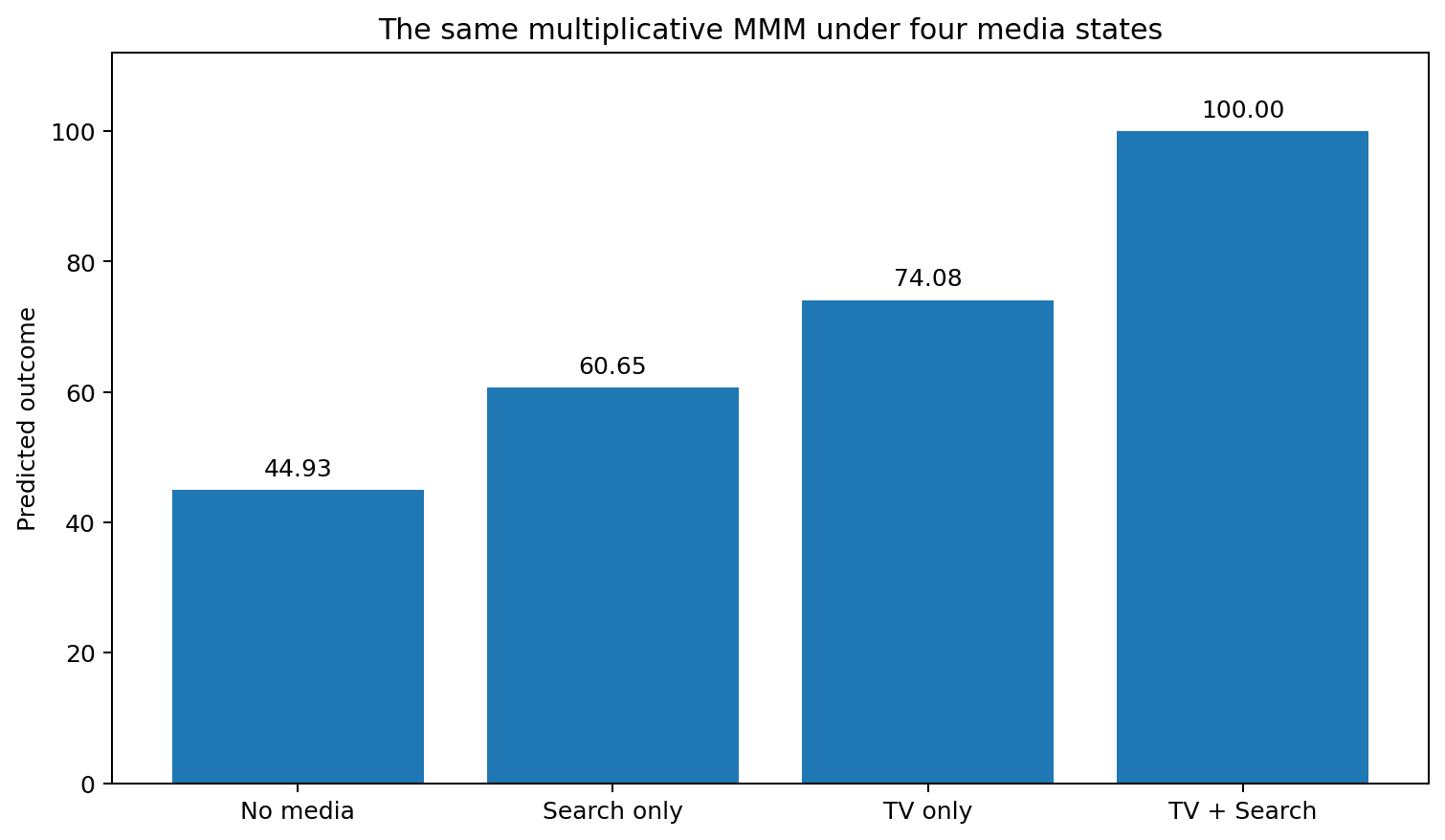
This is the first visual clue that attribution will be order-dependent. Start from the baseline and add TV first: sales go from 44.93 to 74.08, so TV appears to add about 29.15 units. Then add Search: 74.08 to 100, so Search appears to add about 25.92 units.
Reverse the order and the numbers change. Add Search first: 44.93 to 60.65, so Search now appears to add about 15.72 units. Then add TV: 60.65 to 100, so TV now appears to add about 39.35 units. Same model. Same prediction. Different additive story.
Why one-at-a-time removal overcounts
A common contribution calculation removes each channel from the full fitted prediction while leaving everything else active. For player c:
R_c = μ × (1 − exp(−q_c))

R_TV     = 100 × (1 − e^−0.5) = 39.35
R_Search = 100 × (1 − e^−0.3) = 25.92
Add them and you get 65.27. But the true joint media lift is only 100 − 44.93 = 55.07. The difference, 10.20 units, is not real additional sales. It is overlap created by the multiplicative structure. Each one-at-a-time removal calculation gives the removed channel credit for outcome that is partly created jointly with the other active channel.
This makes removal lift useful for a counterfactual question, “what happens to the fitted outcome if I remove this channel while leaving everything else unchanged?”, but it does not automatically make it a valid additive decomposition.
The main decomposition choices
There is no need to treat every method as a competitor. They answer different questions.
1. Raw one-at-a-time removal
R_c = μ × (1 − e^−q_c)Benefits: very simple; intuitive counterfactual; useful for “remove this channel” scenario analysis; deterministic. Weakness: the values generally do not sum to the joint lift. Use it when the removal counterfactual itself is what you want. Do not stack the values and assume they form a unique contribution bridge.
2. Normalised removal
A simple reporting fix is to preserve the relative removal values but scale them to the known total lift:
R̃_c = R_c × L / Σ R_jThis guarantees the values sum to L. Benefits: simple; deterministic; efficient by construction; often close to Shapley when effects are small and positive. Weaknesses: the normalisation is a convention; it can behave poorly when positive and negative effects coexist; and it does not average over the different interaction contexts in which a player can appear.
3. Sequential attribution
Choose one ordering and add or remove players one at a time. Every sequence telescopes exactly to the total lift. Benefits: exactly efficient; easy to explain; can be appropriate if there is a genuinely meaningful causal or operational order. Weakness: change the order and you change the attribution. If “TV before Search” has no substantive meaning, the ordering is arbitrary.
4. Standard discrete Shapley
Shapley removes the arbitrary ordering by averaging a player’s marginal contribution over all possible orderings. The mental picture: each player moves from its reference value to its observed value as one discrete step, and we average that step’s impact over every context the other players can create. Define the value of a coalition S of active players as:
v(S) = μ × (1 − exp(−Σ q_c for c in S))The marginal contribution of player c to coalition S is v(S ∪ {c}) − v(S). With t_j = e^−q_j, the marginal simplifies to μ × (1 − t_c) × ∏ t_j for j in S. The standard Shapley value averages that marginal over all positions and coalitions.
Benefits: exactly efficient; symmetric; no arbitrary fixed ordering; explicit treatment of multiplicative overlap; a strong choice when players are naturally treated as discrete components. Weaknesses: exact generic Shapley can be computationally expensive; interpretation is based on switching whole players between reference and observed states; and for approximate permutation Shapley, the split has Monte Carlo noise.
For this particular multiplicative game, exact calculation is much easier than generic 2ⁿ coalition enumeration. The product structure gives a closed form through elementary symmetric polynomials, and an equivalent integral representation that turns out to be the right way to compute it. We return to the computation later in the post.
5. Permutation Shapley
When exact calculation is inconvenient, sample random player orderings. A useful variance-reduction strategy is antithetic pairing: draw a random permutation, then also evaluate its reverse.
TV -> Search -> Social -> Price
Price -> Social -> Search -> TV
Each individual ordering already telescopes exactly to the joint lift. Therefore the sampled average remains exactly efficient at any sample size. Sampling noise only changes how that fixed total is divided between players.
Benefits: targets standard discrete Shapley; easy to scale; exactly efficient even with a finite sample; antithetic pairing reduces first-mover and last-mover imbalance. Weakness: the player-level split is approximate until enough orderings are sampled.
6. Aumann-Shapley
Aumann-Shapley takes a different view, and it is important to be clear that it is a different attribution definition, not a faster estimator of discrete Shapley. Standard Shapley treats a player as indivisible: it is either at its reference state or at its observed state, and its marginal contribution is averaged over all discrete orderings. Aumann-Shapley treats the effects as continuously divisible: imagine all player effects gradually moving from reference to observed values together along a continuous path, and integrate each player’s marginal effect along that path. For this model, with Q = Σ q_c, that integral has a closed form:
φ_c = μ × q_c × (1 − e^−Q) / Q

// equivalently, when Q ≠ 0:
φ_c = (q_c / Q) × L
So the apparently simple rule “allocate lift proportional to q” is not merely a heuristic here. It is the exact Aumann-Shapley allocation for this path.
Benefits: exact closed form; deterministic; essentially O(n); no Monte Carlo error; exactly efficient; natural when model effects are thought of as continuously moving away from a reference point. Caveat: because it is a different attribution definition, its divergence from discrete Shapley is not an error to be fixed; it is a difference in the counterfactual being described. That distinction can become material when positive and negative effects coexist, as we will see. Near Q = 0, the implementation should use the stable limit (1 − e^−Q)/Q → 1 rather than naively dividing by a tiny number.
7. Equal split
Finally, we can divide the joint lift equally among all players. This is useful as a benchmark because it is efficient and obviously ignores the modelled effect sizes. It is not a serious attribution proposal, but it helps put the other allocation differences in context.
Back to TV and Search
Here is what the methods say for our two-channel example.
| Method | TV | Paid Search | Total |
|---|---|---|---|
| Exact discrete Shapley | 34.25 | 20.82 | 55.07 |
| Aumann-Shapley | 34.42 | 20.65 | 55.07 |
| Normalised removal | 33.20 | 21.87 | 55.07 |
| Raw removal | 39.35 | 25.92 | 65.27 |
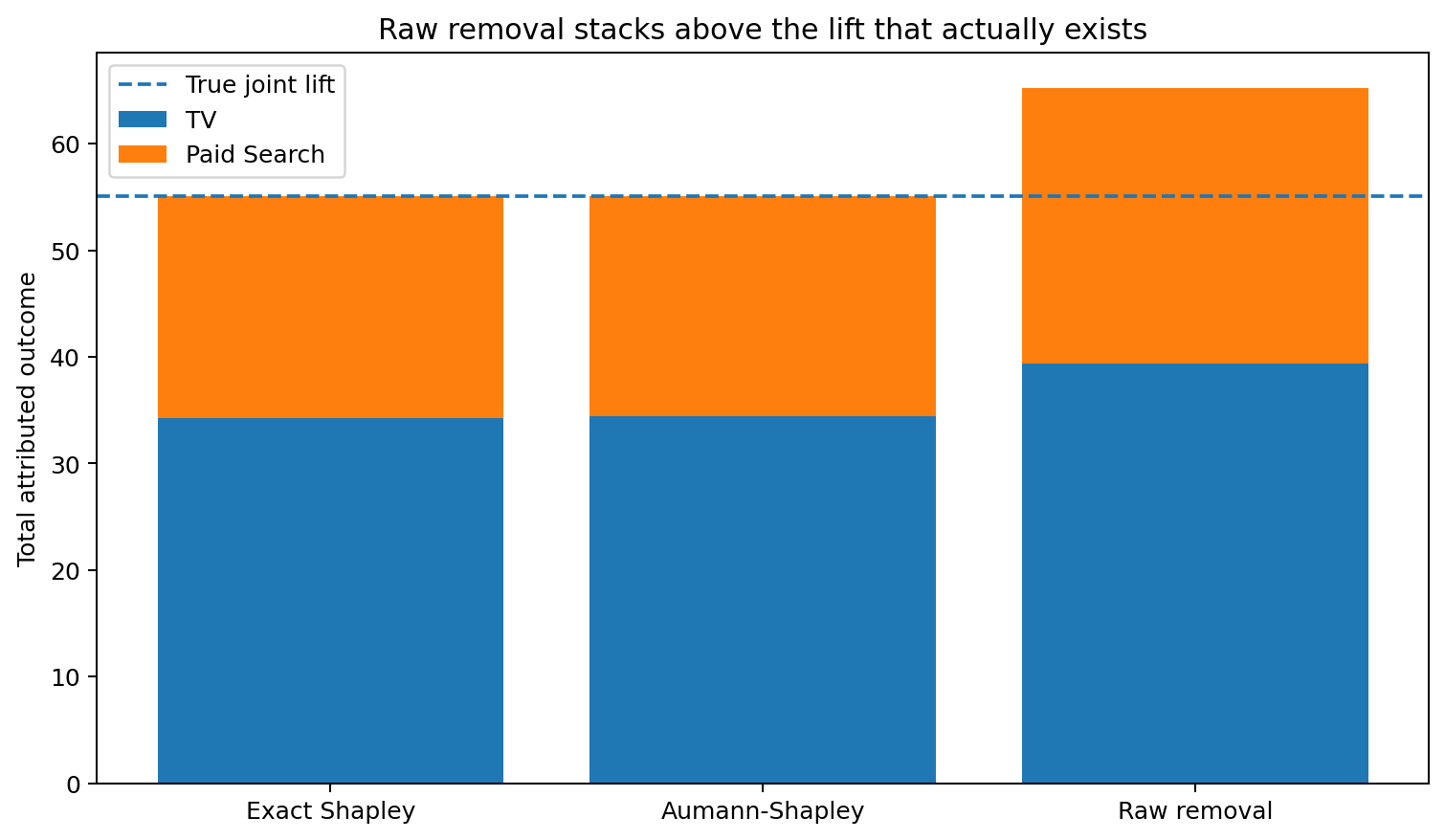
Standard Shapley and Aumann-Shapley are very close here, but they are close for a reason: both effects are positive and moderate in size. That does not mean they are interchangeable.
What about controls that should not go to zero?
Media usually has a natural zero-spend reference. Controls often do not. Suppose a fitted price effect is q_price = 0.7, but the agreed reference level corresponds to q_ref = 0.5. The attribution player should be the difference:
q*_price = q_price − q_ref = 0.7 − 0.5 = 0.2The reference component is absorbed into the baseline. So “remove price” should mean “move price to its reference level”, not “set the price variable to zero”. This matters for every decomposition method. Attribution should operate on the effective effects relative to reference, not blindly on the raw fitted control terms.
Benchmark design
We now move from two channels to as many as 40 players. The benchmark is deliberately controlled. For the positive-only experiment:
- baseline outcome is 100;
- the total log effect is fixed at
Q = 1.2; - therefore the fitted outcome and total lift stay fixed as player count increases;
- individual player effects are heterogeneous but all positive;
- the number of players increases from 2 to 40;
- exact discrete Shapley is computed with two independent engines: the Owen multilinear-extension integral evaluated with Gauss-Legendre quadrature (the production route) and the elementary-symmetric-polynomial formula (retained as a cross-check);
- 128-permutation Shapley uses 64 random permutations plus their 64 reverses;
- the permutation experiment is repeated 200 times at each player count;
- the Gauss-Legendre engine is checked against brute-force permutation enumeration for models up to 8 players and against the elementary-symmetric-polynomial implementation at 20 players, with agreement at machine precision (below 10⁻¹⁴ in the supplied validation run), and its efficiency (contributions summing to the joint lift) is verified at machine precision up to 200 players, including strongly negative effects.
Every method is compared against exact discrete Shapley using the same distance: the total absolute allocation difference, expressed as a percentage of joint lift:
allocation difference = 100 × Σ |φ̂_c − φ_c(exact)| / LThe formula is the same for every method, but what the number means depends entirely on which method it is applied to:
- For permutation Shapley, the number really is approximation error. Permutation Shapley is an estimator of exact discrete Shapley: it targets the same definition, and its distance from that target is Monte Carlo noise that shrinks as more orderings are sampled.
- For Aumann-Shapley, normalised removal, fixed order and equal split, the number is an allocation difference between attribution conventions. These methods are not estimating discrete Shapley; they are answering differently-posed counterfactual questions, so calling their distance an “error” would be a category mistake. More computation will never make it smaller.
The experiment is not claiming that discrete Shapley is a physically observable “true” channel decomposition. The only uniquely known truth from the multiplicative model is the joint lift. Throughout this post, “error” is reserved for permutation Shapley, the one method explicitly approximating the same target, and every other comparison is described as an allocation or decomposition difference.
Benchmark 1: positive effects from 2 to 40 players
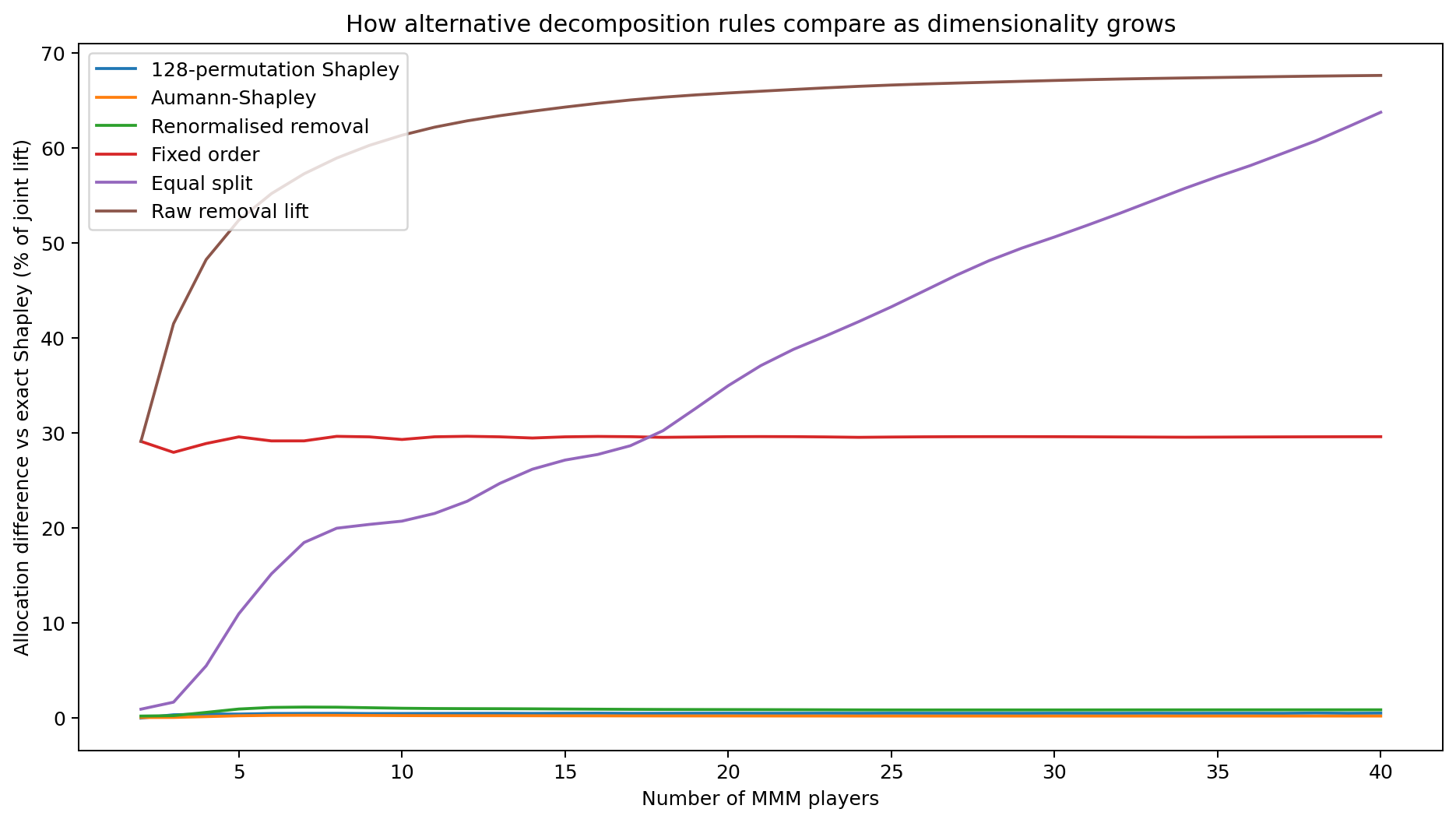
The scale of the chart makes the main result obvious. Raw removal becomes very far from an additive decomposition of the total. Equal splitting also becomes increasingly unlike the model-sensitive allocations. A fixed ordering remains exactly efficient, but produces a very different player split. The three closer methods deserve a zoomed view.
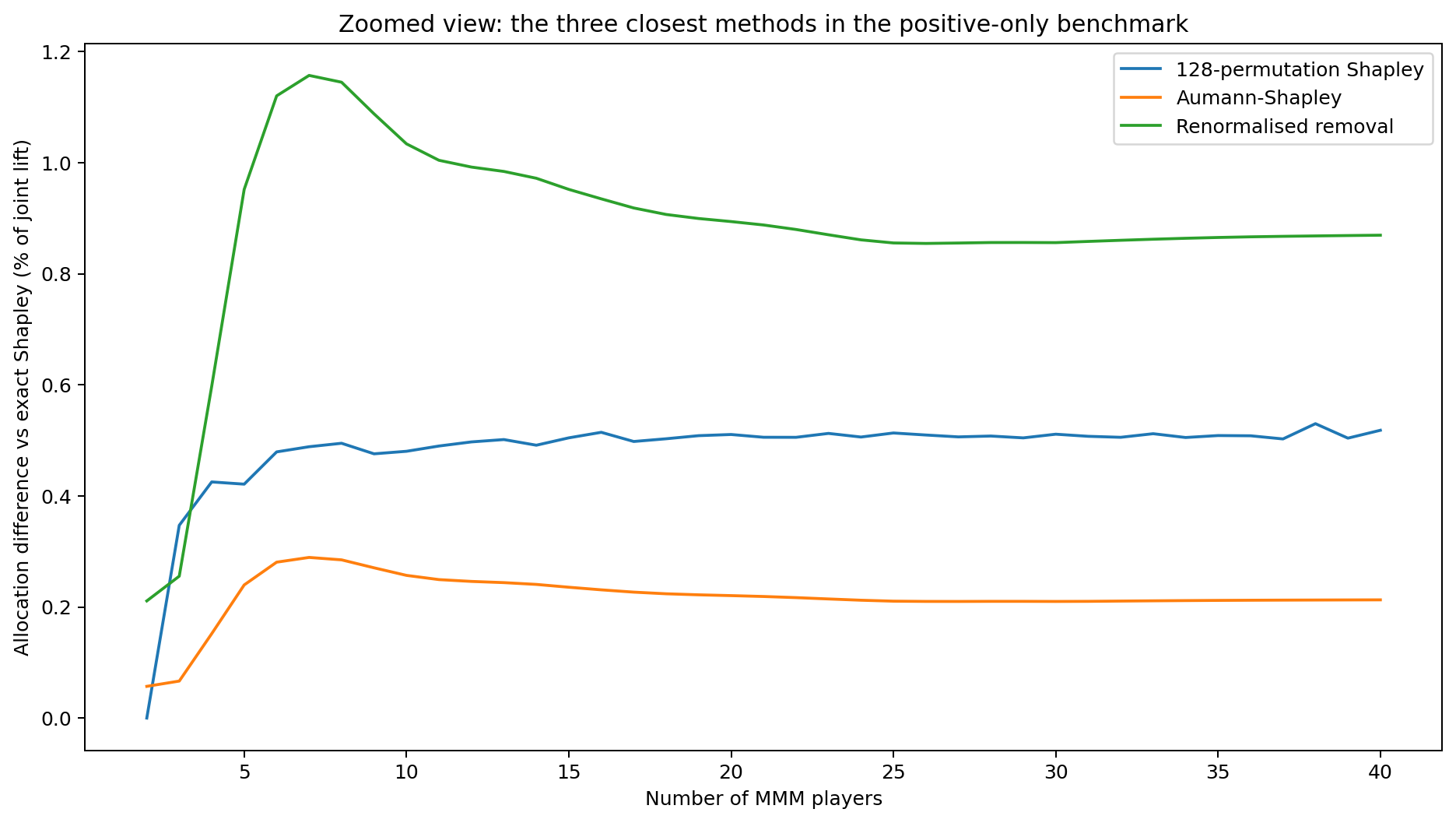
At 40 players:
| Method | Allocation difference vs exact discrete Shapley |
|---|---|
| Aumann-Shapley | 0.213% |
| 128-permutation Shapley, median | 0.518% |
| 128-permutation Shapley, 95th percentile | 0.654% |
| Normalised removal | 0.869% |
| Fixed order | 29.621% |
| Equal split | 63.775% |
| Raw removal lift | 67.655% |
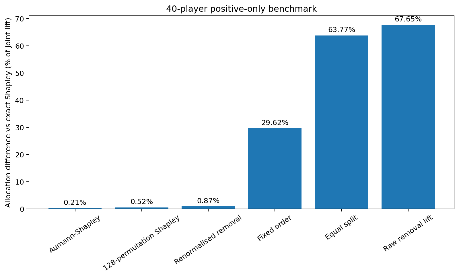
Aumann-Shapley happens to sit closer to exact discrete Shapley than a 128-ordering permutation estimate in this positive-only setup: a 0.213% allocation difference. That should not be read as “Aumann-Shapley is a better estimator than permutation Shapley”, because Aumann-Shapley is not an estimator of discrete Shapley at all. The 128-permutation method targets discrete Shapley, and its 0.52% median error can be driven down by sampling more orderings. Aumann-Shapley is a different attribution rule that happens to produce a very similar allocation under these friendly conditions. Its small distance from discrete Shapley is structural, and more computation will not change it, because it is answering a different question.
Benchmark 2: permutation error falls with more orderings
The 40-player positive model gives us a clean test of Monte Carlo convergence.
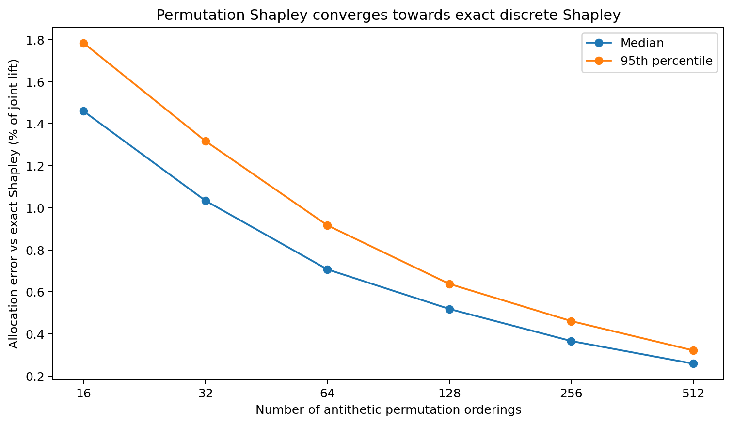
| Orderings | Median allocation error | 95th percentile |
|---|---|---|
| 16 | 1.460% | 1.784% |
| 32 | 1.034% | 1.318% |
| 64 | 0.707% | 0.917% |
| 128 | 0.519% | 0.638% |
| 256 | 0.366% | 0.461% |
| 512 | 0.259% | 0.322% |
At 128 orderings the median split error is about 0.52% of joint lift, with a 95th percentile around 0.65%. At 512 orderings the median falls to about 0.26%. This is the one place in the post where “error” is exactly the right word: permutation Shapley is estimating discrete Shapley, and this chart shows the estimate converging on its target. Note that these are simulation measurements of the sampling estimator; as described later in the post, SIMBA now computes exact Shapley directly at every realistic player count, and keeps this estimator as a validation oracle and extreme-scale fallback.
Permutation sampling never loses the total lift. Every sampled ordering telescopes to exactly the same joint incremental lift, so the sum of channel contributions equals the total at any sample size. The approximation error concerns only how that fixed total is distributed across players (who gets how much credit), never how much total credit exists.
Benchmark 3: positive and negative effects
The positive-only experiment is deliberately friendly to Aumann-Shapley. As the number of players grows while total Q stays fixed, individual effects become smaller, and locally 1 − e^−q ≈ q. In that regime several sensible decomposition rules naturally converge on similar allocations; agreement is cheap. So we need a harder test. The mixed-sign benchmark keeps 40 players and total Q = 1.2, but uses 23 positive effects and 17 negative effects. This is the configuration that real MMMs actually live in once price, distribution gaps, stock-outs and negative events sit alongside media.
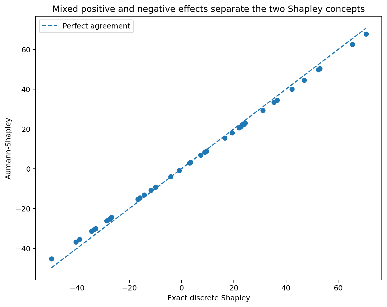
The scatter still looks broadly aligned because the methods agree on direction and much of the magnitude. The more revealing view is the player-level difference:
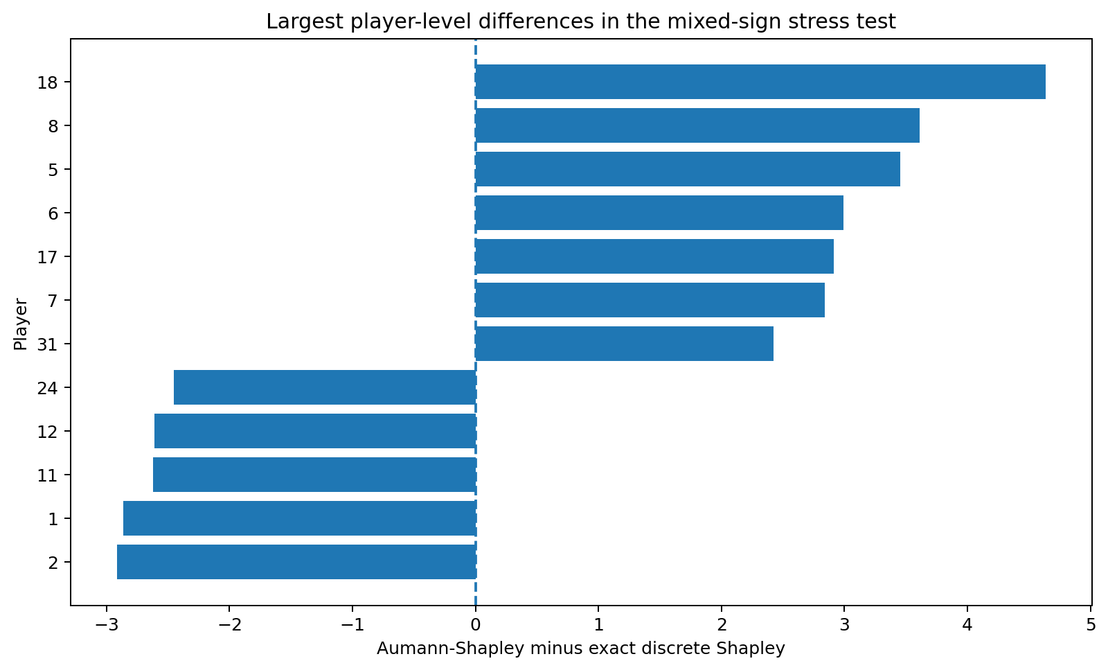
Now the distinction between standard discrete Shapley and Aumann-Shapley becomes much more visible.
| Method | Allocation difference vs exact discrete Shapley |
|---|---|
| 128-permutation Shapley | 6.026% |
| Aumann-Shapley | 30.564% |
| Renormalised removal | 204.109% |
| Raw removal lift | 255.025% |
| Fixed order | 306.295% |
| Equal split | 445.946% |
In the mixed-sign stress test, Aumann-Shapley and discrete Shapley differed by 30.6% of joint lift in aggregate allocation, despite reconciling exactly to the same total incremental outcome. The difference reflects their counterfactual definitions, not a failure of the underlying MMM. Standard Shapley asks: what is this player’s marginal contribution when it enters every possible discrete coalition of the other players? Aumann-Shapley asks: what is this player’s accumulated marginal contribution as all effects move continuously from reference to observed values together? When strong positive and negative effects coexist, those are genuinely different questions, and the choice between them is a counterfactual modelling choice, not a computational optimisation.
It is worth being very careful about what that 30.6% number is. It is calculated as the sum of absolute player-level differences between the two allocations, divided by the total joint lift: a measure of how differently two valid attribution philosophies divide the same total. The average player-level relative difference in this experiment was approximately 7%. The headline number does not mean:
- the MMM prediction was 30% wrong;
- the total incremental contribution was wrong;
- ROI was wrong by 30%;
- each model component differed by 30%.
Both methods reconciled exactly to the same total incremental outcome. The number describes the division of credit, nothing else.
The 128-permutation estimator is the one row in that table where “error” applies: it landed about 6% away from its target in this deliberately difficult setup: a genuine approximation error, and one that more orderings would reduce. Even there, the total contribution remained exactly correct; only the split was noisy.
The same stress test also exposes a weakness in normalised removal. With mixed signs, forcing one-at-a-time removal values to sum correctly can heavily distort individual allocations. A method that looks harmless in a positive-only media model can become unstable when controls and events introduce negative effects.
So which method should an MMM use?
There is no universal winner because the methods encode different semantics.
Use raw removal when the question is genuinely a removal scenario
If the business question is “what happens if this channel disappears while the rest of the plan remains unchanged?”, then one-at-a-time removal is exactly the relevant counterfactual. Just do not mistake a collection of those counterfactuals for an additive decomposition.
Use discrete Shapley when players are treated as whole components
If TV, Search, price and a holiday effect are treated as discrete model components and the goal is a fair additive decomposition without arbitrary ordering, standard Shapley is a strong choice. For this multiplicative game, the product structure can be exploited to calculate exact Shapley much more efficiently than generic subset enumeration; as we show below, exact values are now practical at every realistic player count. Where sampling is still used, antithetic permutation sampling has a useful property: the split may be noisy, but the total is exactly right at every sample size.
Use Aumann-Shapley when the continuous path is the right counterfactual
Media intensity is not naturally binary. Spend, impressions and transformed media effects are continuous. If the meaningful thought experiment is to move every component gradually from its reference state to its observed state, Aumann-Shapley is particularly attractive. For this model it is also exceptionally simple: no permutations, no sampling noise, one closed-form line. But the mixed-sign benchmark shows why the attribution definition must be named explicitly. Aumann-Shapley should not be silently presented as “standard Shapley, but faster”.
Treat normalised removal as a pragmatic reporting rule
It can work surprisingly well when all effects are positive and relatively small. It is easy to calculate and easy to explain. But it becomes much less appealing once negative effects and reference-point controls are part of the decomposition.
How SIMBA decomposes multiplicative models
SIMBA’s preferred general attribution convention for multiplicative models is discrete Shapley. Not because Shapley is fashionable, but because of what it does structurally. Discrete Shapley:
- treats each model component as a player;
- evaluates its marginal impact across the different contexts created by the other players;
- removes dependence on one arbitrary sequential ordering;
- allocates multiplicative overlap rather than duplicating it;
- exactly reconciles contributions to the joint incremental lift;
- works naturally for media, controls, events and other components;
- remains meaningful when positive and negative effects coexist.
That last point is exactly what the mixed-sign benchmark was probing. And for controls with reference points, Shapley is applied to the effective effect:
q_effective = q − q_referenceso “removing” a control means moving it back to its defined reference state, not setting the raw variable to zero. Aumann-Shapley remains a legitimate, elegant alternative: deterministic, closed form, and near-indistinguishable from discrete Shapley in positive-effect settings. But remember what the stress test showed: with mixed positive and negative effects the two conventions materially diverge, by roughly 30% of total allocation in this post's own 23-positive/17-negative simulation. That is precisely when naming the convention matters. Aumann-Shapley is selectable in SIMBA under that name. The implementation follows the recipe above: −expm1(−Q)/Q with a Taylor series below |Q| < 10⁻³ carrying the limit of 1 at Q = 0, so exact cancellation, say q = [0.5, −0.5] with μ = 100, yields [+50, −50] with zero total and no numerical surprises. The requirement is simply that whichever convention is used is named, so a contribution chart can never be mistaken for a unique model readout.
The bigger lesson
There is a temptation in MMM reporting to think of channel contribution as if it were another posterior parameter waiting to be read from the model. In a multiplicative model, it is not. The model tells us the fitted outcome, the baseline or reference outcome, the log-scale effects, and the joint incremental lift. To produce a stacked contribution chart, we add one more decision: how should interaction created by multiplication be allocated across the players?
Raw removal leaves that overlap duplicated. Sequential attribution gives it to players according to one ordering. Discrete Shapley averages it across every ordering. Aumann-Shapley distributes it along a continuous path. Those are different, defensible answers to different questions. The important thing is not to hide the choice.
A contribution chart from a multiplicative MMM is not just a direct readout of the model. It is the combination of the model and an attribution convention. The total joint lift is identified by the model. The player-level additive decomposition depends on the convention. SIMBA uses Shapley-style decomposition so multiplicative overlap is allocated explicitly and channel contributions reconcile to the model’s joint incremental lift.
Exact Shapley at scale: how SIMBA computes it now
When this post was first published, this section described future work: use exact Shapley for small player counts, switch to permutation sampling for larger ones, and hope a stable O(n²) exact route could be found. That work has now shipped in SIMBA's attribution engine, and it changed the architecture. Exact discrete Shapley is now computed for every model up to 200 players. Permutation sampling (unchanged: 128 orderings as 64 antithetic pairs, with a fixed seed) is retained only as a validation oracle and as a fallback beyond 200 players. In practice, every realistic MMM fit now gets exact, deterministic Shapley values with zero sampling error. The permutation error statistics quoted earlier in this post are therefore simulation measurements of the fallback estimator, not descriptions of production behaviour.
The route that made this possible is the Owen multilinear-extension integral. For player c:
φ_c = μ × (1 − t_c) × ∫₀¹ ∏_{j≠c} (1 − x + x·t_j) dx, t_j = e^−q_jevaluated with Gauss-Legendre quadrature. Two properties make this the right computation. First, it is exact, not approximate: the integrand is a polynomial of degree n − 1 in x, so ⌈n/2⌉ quadrature nodes evaluate the integral exactly. Second, it is numerically stable: every factor (1 − x + x·t_j) is strictly positive on [0, 1], so the per-player division that removes player c involves no cancellation. The cost is O(n²) vectorised array operations, and accuracy is machine precision, verified to n = 200 including strongly negative effects (t up to about 8). Mathematically it is the same closed form as the elementary-symmetric-polynomial identity given earlier, via ∫₀¹ xᵏ(1 − x)ⁿ⁻¹⁻ᵏ dx = k!(n−1−k)!/n!, which is exactly the Shapley coalition weight; the ESP formula is retained in the benchmark code as an independent cross-check.
A warning about the tempting shortcut. An earlier version of this post floated a potential O(n²) implementation of the ESP formula itself: compute the global polynomial P(z) = ∏_j (1 + t_j·z) once, then recover each player’s excluded-player polynomials by dividing out its factor with the recurrence e_k^(−c) = E_k − t_c × e_(k−1)^(−c). This has now been tested, and it is catastrophically numerically unstable. Do not implement it. The rounding error amplifies at every deflation step and the global coefficients grow combinatorially: in the benchmark package’s positive-only test the relative error is already around 10⁻⁷ by 40 players, and the results are wrong by many orders of magnitude at 80. The Gauss-Legendre integral achieves the same O(n²) cost with machine-precision accuracy, which is why it is the production route. The downloadable code keeps the deflation variant as a clearly-marked negative example so the blow-up can be reproduced.
How does exact compare with sampling in practice? The engine was benchmarked over a full posterior grid of 156 dates × 1,000 draws, meaning the allocation runs once per draw and date; times are wall-clock for the whole grid:
| Players | Old O(n³) ESP | Gauss-Legendre exact | 128-permutation | Permutation split error |
|---|---|---|---|---|
| 5 | 0.12s | 0.08s | 4.9s | 0.23% |
| 12 | 1.56s | 0.37s | 12.2s | 0.87% |
| 20 | 3.8s | 0.46s | 14.3s | 1.9% |
| 40 | n/a | 1.1s | 27.5s | 4.4% |
| 100 | n/a | 8.9s | 73s | 12.8% |
| 200 | n/a | 35s | 171s | 20.2% |
The reading is unambiguous: exact now dominates sampling on both speed and accuracy at every player count. At 40 players, even 512 permutations retain roughly 2.3% split error while taking around 18 times the exact method’s runtime. The old exact-versus-sampling trade-off, precision against cost, simply no longer exists for this characteristic function. The cutoff that used to sit at 12 players now sits at 200, which is beyond any realistic MMM.
The decomposition layer now looks like this, with both conventions first-class and cheap:
Multiplicative MMM
        |
   effective q
        |
        +-------------------------+
        |                         |
Exact discrete Shapley      Aumann-Shapley
Owen + Gauss-Legendre       closed form O(n)
O(n²), all n ≤ 200          proportional to q
        |                         |
        +-------------+-----------+
                      |
             transparent metadata

(128 antithetic permutations: validation oracle,
 and fallback beyond 200 players)
A practical reporting standard
For a transparent multiplicative MMM, I would want every contribution export to carry enough metadata to reproduce its meaning:
{
  "attribution_method": "discrete_shapley",
  "method": "exact",
  "algorithm": "owen_gauss_legendre"
}
or, for the sampling fallback:
{
  "attribution_method": "discrete_shapley",
  "method": "permutation",
  "algorithm": "antithetic_permutation",
  "n_permutations": 128,
  "seed": 20260813
}
or:
{
  "attribution_method": "aumann_shapley",
  "method": "closed_form",
  "algorithm": "proportional_expm1"
}
This is what SIMBA's attribution engine now declares on every fit: the convention, the estimation method, and the algorithm, with the permutation count and seed included whenever sampling is involved.
Controls should also carry their attribution reference levels. The attribution method should be part of the model metadata, alongside the model specification itself. That turns a contribution chart from a black-box output into a reproducible modelling decision. And that is ultimately the point. A sophisticated MMM should not only tell you what the contribution numbers are. It should make it possible to understand why those numbers add up the way they do. This is the same transparency principle behind the rest of the SIMBA Bayesian MMM workflow.
Reproduce the benchmarks
Every number and figure in this post is generated from a fixed random seed by a small, self-contained code package. Download the benchmark package. It contains:
- exact discrete Shapley via the Owen integral with Gauss-Legendre quadrature (the production route) and via elementary symmetric polynomials (the independent cross-check);
- the unstable ESP deflation shortcut, kept as a clearly-marked negative example, with a test that reproduces its error blow-up;
- brute-force Shapley validation for small models, and machine-precision efficiency checks up to 200 players;
- 128-ordering antithetic permutation Shapley;
- Aumann-Shapley;
- raw and normalised removal;
- fixed-order sequential attribution;
- the positive-only 2-to-40-player benchmark;
- the mixed-sign stress test;
- permutation convergence tests;
- every CSV used in this post.
pip install -r requirements.txt
python code/run_all.py
If you want to talk through how your MMM decomposes contributions, or how SIMBA reports attribution methodology explicitly, book a call. For the modelling side of multiplicative MMMs, see Bayesian MMM Explained.